Ghosts in the Machine
Why AI language models invent references that never existed — and how computers actually match citations correctly.
Introduction: The Confident Liar
Ask a modern AI chatbot for five scientific papers on almost any topic and you will get a beautifully formatted list: plausible author names, a real-sounding journal, a volume and page range, even a DOI that has the right shape. There is just one problem. Some of those papers have never existed. The authors are real people who never wrote that paper together; the journal is real but never published that article; the DOI resolves to nothing, or to something completely different.
This is not a rare glitch. It is one of the most consistent and well-documented failure modes of large language models (LLMs), and it has already produced sanctioned lawyers, rejected conference papers, and a new academic sub-discipline devoted to catching “phantom” citations. This article explains two things. First, why this happens — the machinery of language models that makes a fabricated citation the same kind of object, internally, as a real one. Second, how the problem is actually solved — the decades-old and rapidly evolving field of citation matching, entity resolution, and retrieval that lets a computer reliably connect a messy human reference to a real record in a database.
We start where anyone can follow along and go progressively deeper. A curious reader can stop after the first couple of sections with a solid mental model. A scientist or engineer can keep reading into tokenization internals, embedding mathematics, approximate-nearest-neighbor search, rank fusion, and calibration. Each section is labeled with roughly how deep it goes.
Part 1 — The Problem: Why LLMs Fabricate References
Depth: beginner → intermediate
What “hallucination” actually means
In AI, a hallucination is confident output that is not grounded in reality: an invented statistic, a misquoted source, a fabricated legal case, or — our focus — a citation to a paper that does not exist. The unsettling part is not that the machine is wrong; all tools make errors. It is that the machine is wrong with total confidence, in fluent, authoritative, correctly formatted prose. A hallucinated citation looks exactly like a real one because looking real is literally the only thing the model was trained to do.
The single most important sentence to internalize comes from William Walters and Esther Wilder, who published the first large systematic study of the phenomenon in Scientific Reports in 2023:
“It is important to realize, however, that ChatGPT is fundamentally not an information-processing tool, but a language-processing tool. It mimics the texts — not necessarily the substantive content — found in its information base.”
That distinction — language processor, not information processor — is the entire story in miniature. Keep it in mind through everything that follows.
How a fake reference is born, token by token
To see the mechanism, watch a language model “write” a citation. An LLM generates text one small piece (a token — Part 2 explains these precisely) at a time, each piece chosen because it is statistically probable given everything written so far. The model has read millions of bibliographies during training, so it knows the shape of a reference perfectly: after a surname comes an initial; after a title about transformers comes a venue like a machine-learning conference; after “pp.” come plausible page numbers.
So the model produces, say: “Chen, L., & Martinez, R. (2019). Graph Neural Approaches to Bibliographic Entity Matching. Proceedings of SIGIR, 412–421.” Perfectly formatted. Grammatically ideal. Completely invented. Every part is statistically plausible; the whole thing never existed. And — this is the crucial point — the model cannot tell the difference. Generating a real memorized reference and confabulating a fake one are the same internal operation: produce plausible next tokens. There is no flag inside that says “retrieved” versus “invented,” because nothing was ever retrieved. There is no database inside the model — only billions of numerical weights storing statistical patterns.
The documented scale of the problem
The foundational study. Walters & Wilder had ChatGPT-3.5 and ChatGPT-4 produce short literature reviews on 42 topics, then checked all 636 resulting citations. The result: 55% of GPT-3.5’s citations were entirely fabricated, versus 18% for GPT-4. Among the citations that did refer to real papers, 43% (GPT-3.5) and 24% (GPT-4) still contained substantive errors — wrong volume, wrong pages, wrong year. Even the “real” citations were frequently mangled. An earlier medical case report (Alkaissi & McFarlane, 2023) found that all five references ChatGPT generated for one topic were nonexistent, with PubMed IDs pointing to unrelated papers.
It reached the top of the field. In January 2026, the AI-detection company GPTZero reported scanning 4,841 of the 5,290 papers accepted to NeurIPS 2025 — one of the world’s most prestigious machine-learning conferences — and finding 100 verified hallucinated citations across 53 accepted papers (about 1% of acceptances). Each of those papers had passed at least three expert reviewers. With a 24.5% acceptance rate, each had beaten out thousands of competitors while containing fabricated references. The fakes included invented authors, nonexistent articles, fake DOIs, and “amalgamations” — real fragments fused into fictional wholes.
It is growing exponentially. The most rigorous longitudinal audit (Sakai, Kamigaito & Watanabe; ACL 2026) examined 17,842 papers across the ACL, NAACL and EMNLP conferences for 2024–2025. Papers containing at least one hallucinated citation jumped from 20 in 2024 to 275 in 2025 — the affected share rising roughly tenfold, from 0.28% to 2.59%, reaching 3.7% at EMNLP 2025 alone. A separate large-scale audit that leveraged 111 million references across 2.5 million papers produced a conservative estimate of ~147,000 hallucinated citations entering the scientific literature in 2025 alone.
Conferences are fighting back. ICLR 2026 instituted desk-rejection for papers with confirmed hallucinated references — an automated detector flagged candidates, and every flagged reference was manually verified by at least three humans before rejection. ACL 2026 announced during camera-ready checks that it had identified and rejected over 100 papers citing non-existent literature, stating that “preserving the integrity and reliability of the ACL proceedings is our responsibility.”
The legal reckoning
Mata v. Avianca (2023) is the landmark. A New York attorney used ChatGPT to research a brief and filed six entirely fabricated judicial opinions — complete with invented quotes, fake docket numbers, and imaginary judges. When opposing counsel could not find the cases, the attorney asked ChatGPT whether they were real; it assured him they were — a second hallucination stacked on the first. The court sanctioned the attorneys and their firm $5,000, finding “subjective bad faith” — not for using AI, but for failing to verify and then doubling down.
The problem exploded from there. The most comprehensive public tracker of court decisions involving AI-hallucinated content (maintained by legal researcher Damien Charlotin) has logged over 1,700 cases, and its author reports the inflow reached roughly five new cases per day by early 2026. Penalties have escalated: in one 2026 federal appeals decision, two attorneys were fined $15,000 each plus the opposing side’s full fees, the court explaining it chose that amount because “smaller fines have plainly been inadequate.”
Even retrieval doesn’t fully fix it
A natural response: “Just connect the model to a search engine or database.” This architecture — retrieval-augmented generation (RAG) — helps a great deal, but does not eliminate the problem. Stanford’s RegLab tested commercial, retrieval-augmented, legally trained research tools that marketed themselves as hallucination-free. The findings: one leading tool hallucinated on more than 17% of queries; another about 33% — roughly one answer in three; general-purpose GPT-4 hallucinated 43% on the same tasks. A 2026 study of citation URLs found 3–13% of citations produced by “deep research” agents pointed to pages that likely never existed — and agents that generate more citations hallucinate at higher rates.
Retrieval puts real documents in front of the model, but the model still writes the answer itself — and it can ignore, misread, blend, or embellish what it was shown. The data still flows through the model’s generative machinery on its way to you. To truly eliminate fabrication, the architecture must change so that bibliographic data flows around the model — retrieved verbatim from a database, untouched by generation. That inversion is Part 4.
The deep reason: guessing is rewarded
Depth: intermediate
A 2025 OpenAI paper (“Why Language Models Hallucinate”) gave the phenomenon a rigorous statistical grounding: “language models hallucinate because the training and evaluation procedures reward guessing over acknowledging uncertainty.” Two of its arguments matter especially for citations:
- The singleton argument. For facts that appear rarely and follow no learnable pattern, the model’s error rate is bounded below by how many such facts it saw only once. A specific paper’s exact citation string — precise author order, exact DOI suffix, page range — is exactly this kind of arbitrary, low-frequency, high-precision fact. If 20% of such strings appeared once in training, expect at least ~20% hallucination on them.
- The test-taker argument. Benchmarks grade a confident wrong answer the same as “I don’t know” — so training optimizes models to always guess. Asked for an obscure researcher’s birthday “only if you know it,” one leading model produced three different confident wrong dates across three attempts.
There is one more mechanical reason fake citations are so specifically broken — the model’s worst errors cluster in surnames, DOIs, and page numbers. That reason lives one level down, in how text becomes numbers in the first place.
Part 2 — Tokenization: How Text Becomes Numbers
Depth: beginner → deep
Why tokenization exists at all
Computers do not read text; they do arithmetic on numbers. Before a neural network can process the word “cat,” that word must become a number. The component that chops text into pieces and assigns each piece a number is the tokenizer, and the pieces are tokens. Every LLM has one, it runs before the model proper, and its design has surprisingly deep consequences — including for citation accuracy.
A token is an entry in a fixed dictionary called the vocabulary. Each token maps to an integer ID. The sentence “I like cats” might become the IDs [40, 588, 11875]. The model only ever sees those integers. The whole design question is: what should the pieces be? There is a spectrum, and each point on it trades something away.
The taxonomy of tokenization
Character-level. Every character is a token. Vocabulary is tiny (a few hundred symbols) and nothing is ever unknown. But sequences become extremely long — “tokenization” alone is 12 tokens — which is computationally expensive, and the model must learn spelling and word structure from scratch.
Word-level. Every word is a token. Sequences are short and each token is meaningful. But the vocabulary explodes — English has millions of word forms once you count inflections, names, typos, and technical terms (“love,” “loving,” “loved,” “lovingly” are four separate entries). Worse, any word not seen in training becomes an out-of-vocabulary token — an unusable “unknown” — which is catastrophic for names, code, and new coinages.
Subword — the modern standard. Keep common words whole; break rare words into meaningful fragments. “unbelievable” → [un, believ, able]. Common words cost one token; rare ones decompose into known pieces, so nothing is ever truly unknown, and the vocabulary stays manageable (tens of thousands of entries). Three algorithms dominate.
Byte-Pair Encoding (BPE)
Used by the GPT family, Llama, Qwen and many others; adapted for language in 2016 from a 1994 compression algorithm. Training is beautifully simple:
- Start with a base vocabulary of individual characters (or bytes).
- Count all adjacent symbol pairs in the training corpus.
- Merge the single most frequent pair into a new token.
- Repeat until the vocabulary reaches its target size.
WordPiece
Used by BERT and its relatives. Nearly identical to BPE with one twist: instead of merging the most frequent pair, it merges the pair that most increases the likelihood of the training data — roughly, the pair whose combined frequency is highest relative to the product of its parts’ individual frequencies. This favors merges that are genuinely informative rather than merely common. WordPiece marks continuation pieces with “##”: “playing” → [play, ##ing].
Unigram Language Model
Used by T5 and many multilingual models. It works backwards: start with a large superset of candidate subwords, fit a probabilistic model assigning each a probability, then iteratively prune the tokens that contribute least to the corpus likelihood until reaching the target size. Its advantage: it can represent multiple possible segmentations of a word with probabilities — a regularization trick BPE cannot do natively.
SentencePiece and byte-level BPE
SentencePiece is a framework implementing BPE and Unigram in a language-agnostic way: it treats the input as a raw character stream including spaces (encoded as a visible “▁” symbol), so it needs no language-specific pre-splitting — crucial for Japanese or Chinese, which don’t separate words with spaces. Byte-level BPE (GPT-2 onward) uses the 256 possible byte values as the base alphabet instead of Unicode characters. Since all text in every language is ultimately bytes, nothing is ever unknown — worst case, a strange string is spelled out byte by byte. GPT-2’s vocabulary of 50,257 is exactly 256 bytes + 50,000 merges + 1 special token.
The frontier: models without tokenizers
Tokenization is increasingly seen as a brittle necessity, and researchers are attacking it. ByT5 operates directly on raw UTF-8 bytes (robust to typos, but sequences get very long). MambaByte applies a state-space model to raw bytes. Most notably, Meta’s Byte Latent Transformer (late 2024) introduced dynamic patching: bytes are grouped into variable-sized patches whose boundaries are set by prediction difficulty — more compute where text is surprising, less where it is predictable — reportedly matching tokenizer-based models at scale. If this line matures, some failure modes described next may fade. For now, essentially every deployed model tokenizes.
| Model / tokenizer | Scheme | Vocabulary size |
|---|---|---|
| BERT | WordPiece | ~30,000 |
| GPT-2 | byte-level BPE | 50,257 |
| GPT-3.5 / GPT-4 (cl100k_base) | byte-level BPE | ~100,000 |
| GPT-4o / o-series (o200k_base) | byte-level BPE | ~200,000 |
| Llama / Llama 2 | BPE (SentencePiece) | 32,000 |
| Llama 3 | byte-level BPE | 128,000 |
| T5 | Unigram (SentencePiece) | 32,000 |
Larger vocabularies pack more text into fewer tokens (cheaper, faster, better for code and non-English text) but require a bigger embedding table inside the model.
Why tokenization matters for citations specifically
Depth: intermediate
Here is the mechanical link back to Part 1. Consider what a citation is made of: author surnames (many rare, non-English, easily misspelled), a DOI (an arbitrary string like 10.1038/s41598-023-41032-5), page numbers, volumes, years. These are precisely the elements that tokenize badly.
A common word like “the” is one token, reinforced by billions of examples. But an unusual surname fragments into several subword pieces — [No, wo, zin] — that the model must reproduce in exactly the right order, from statistical memory, with nothing to check against. A DOI is worse still: near-random from the model’s perspective, it shatters into a long sequence of digit-and-punctuation tokens with almost no statistical regularity to anchor them. One slip anywhere in the sequence and the identifier is corrupted — and there is no “spell-check against reality” inside a generative model.
Across studies, the title is consistently the most accurately reproduced field of a generated citation, while the DOI is the worst, with numerical metadata (volume, pages) error-prone in between. That is exactly what the tokenization analysis predicts: the model retains the gestalt (frequent, patterned tokens) and corrupts the specifics (rare, arbitrary token sequences). A real author paired with a title they never wrote; a correct journal with a wrong volume; a DOI valid in form pointing nowhere — the signature of pattern storage, not record storage.
Part 3 — Text Embeddings: Turning Meaning into Geometry
Depth: beginner → deep
The beginner’s picture
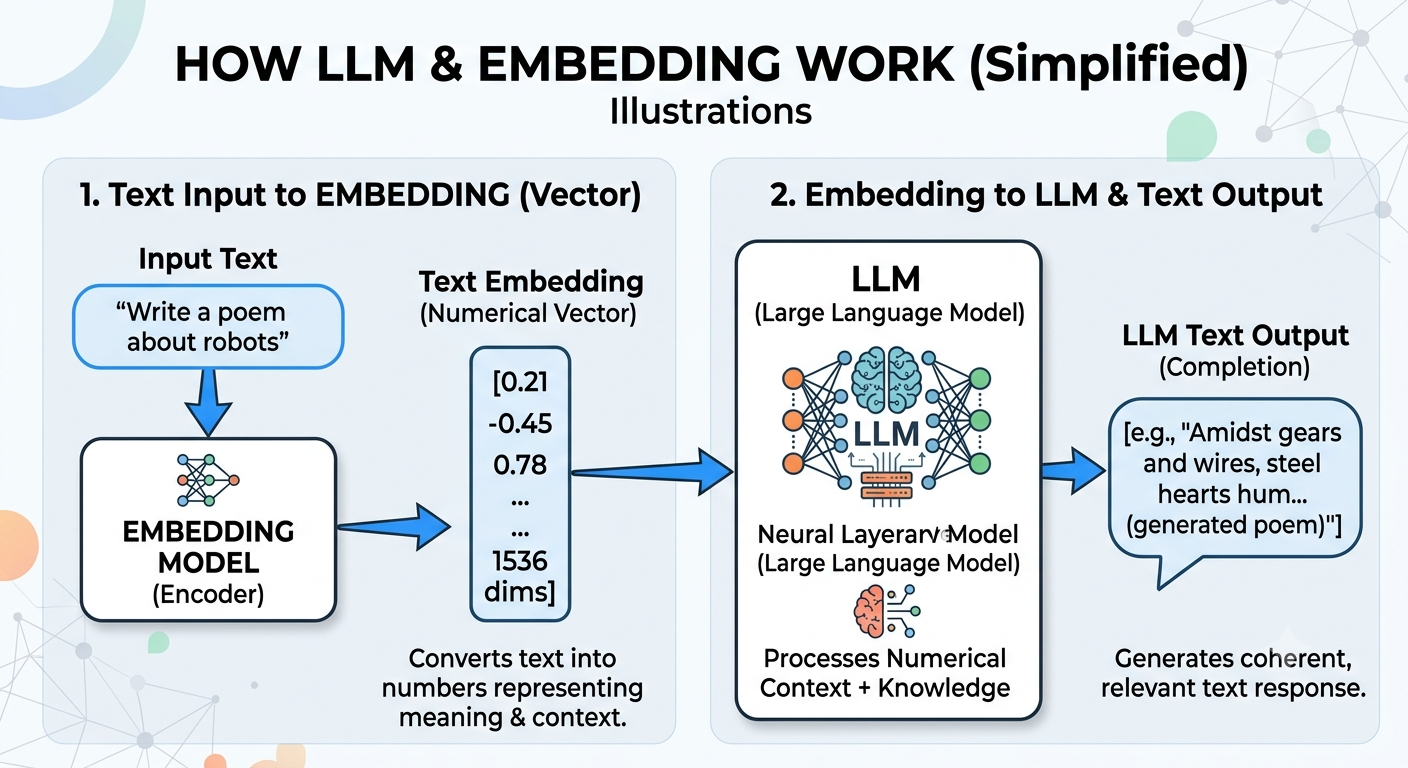
If tokenization turns text into ID numbers, embeddings turn text into meaningful numbers. An embedding is a list of numbers — a vector — that represents the meaning of a word, sentence, or document, positioned in a high-dimensional space so that things with similar meaning sit close together.
Imagine a map where every point is a piece of text. On a good map, “cat,” “kitten,” and “feline” cluster in one neighborhood; “democracy” and “election” cluster far away in another. That is an embedding space — except instead of two dimensions it has hundreds or thousands. Closeness in this space is semantic similarity. This single idea is the foundation of modern search, recommendation, and retrieval: to find documents about a topic, convert the query to a vector and look for nearby document vectors — even when they share no words.
How embeddings are actually produced
Depth: intermediate → deep
For a modern transformer-based embedding model, four steps:
- Tokenize the text into token IDs (Part 2).
- Look up each ID in a learned embedding table — a giant matrix with one row per vocabulary entry — to get an initial vector per token. These starting vectors are context-free: the token “bank” gets the same row whether it means a riverbank or a financial institution.
- Contextualize through transformer layers using attention — the key step. Attention lets each token’s vector be updated by “looking at” every other token and absorbing relevant information. After a few layers, the vector for “bank” in “river bank” has drifted toward water; in “bank account,” toward finance. Meaning becomes contextual.
- Pool the many token vectors into one fixed-size vector for the whole text — either the special [CLS] summary token’s vector, or the mean of all token vectors. The result: a single vector of typically 384, 768 or 1024 numbers representing the entire input.
Measuring similarity: cosine similarity, with a worked example
Once two texts are vectors, similarity is the cosine of the angle between them — direction matters, length doesn’t:
cos(θ) = (A · B) / (‖A‖ ‖B‖) = Σ AᵢBᵢ / ( √ΣAᵢ² · √ΣBᵢ² )It ranges from −1 (opposite) through 0 (unrelated) to +1 (identical direction). A tiny worked example in 2-D: let A = [2, 1], B = [3, 1.5], C = [−1, 2].
- A vs B: dot product = 2×3 + 1×1.5 = 7.5; ‖A‖ = √5 ≈ 2.236; ‖B‖ = √11.25 ≈ 3.354; cosine = 7.5 / (2.236×3.354) ≈ 1.00 — same direction (B is just a longer arrow), maximal similarity.
- A vs C: dot product = 2×(−1) + 1×2 = 0; cosine = 0 — perpendicular, unrelated.
That single number, computed billions of times per second across the industry, is the workhorse of semantic search.
Where “meaning” comes from: nobody assigns it
Why does any of this work? The bedrock is the distributional hypothesis, crystallized by the linguist J.R. Firth in 1957: “You shall know a word by the company it keeps.” Words with similar meanings appear in similar contexts — “dog” and “cat” both live near “pet,” “feed,” “fur,” “vet.” A model trained to predict text from context is therefore forced to give similar words similar vectors: they must be interchangeable in its predictions. Nobody labels synonyms; the statistics of human language do it.
The training objectives are self-supervised — signals extracted from raw text with no human annotation:
- Masked language modeling (BERT): hide a word, train the model to predict it from context.
- Contrastive learning: show pairs that should be close (a question and its answer) and pairs that should be far, and train the model to pull positives together, push negatives apart.
- Triplet loss: with an anchor, a positive and a negative, require anchor–positive to be closer than anchor–negative by a margin.
A perfect example for our topic: the scholarly-document models SPECTER and SPECTER2 are trained on the citation graph itself — if paper A cites paper B, their embeddings are pulled together. SPECTER2 trained on over 6 million citation triplets across 23 fields. The result is a space where related papers cluster, computable from just a title and abstract — enormously useful for matching, and needing no citation data at inference time.
The famous party trick of early embeddings: vector(“king”) − vector(“man”) + vector(“woman”) ≈ vector(“queen”) (word2vec, 2013). Relationships like gender or royalty appeared as consistent directions in the space. The caveat: the effect is real but often overstated — it works cleanly for some relations only, and the standard evaluation quietly excludes the input words from the candidate answers. Treat it as a beautiful illustration, not a law.
Does dimension 42 mean “royalty”? Almost never. Embeddings are distributed representations: meaning is smeared across many dimensions, and any single dimension participates in many unrelated concepts (a phenomenon related to superposition — networks pack more features than they have dimensions by using overlapping combinations). Meaning corresponds to directions through the space, not to individual axes. You compare whole vectors, never inspect single coordinates.
A brief history
| Year | System | What changed |
|---|---|---|
| 2013 | word2vec | Efficient static word vectors; the analogy era |
| 2014 | GloVe | Word vectors from global co-occurrence statistics |
| 2018 | ELMo | First widely used contextual embeddings — same word, different vector per sentence |
| 2018 | BERT | Transformer + masked-word training; a watershed |
| 2019–20 | Sentence-BERT, SPECTER | Good sentence/document-level vectors; SPECTER trained on citation graphs |
| 2022–26 | E5, BGE / BGE-M3, text-embedding-3, Qwen3-Embedding, SPECTER2 | Modern multilingual sentence embeddings; long context; adjustable dimensions; MTEB benchmark standardizes comparison |
Searching millions of vectors in milliseconds
Depth: deep
One scaling problem remains. With 100 million paper embeddings, computing cosine similarity of a query against all of them (exact, “brute-force” search) is too slow for interactive use. The fix is Approximate Nearest Neighbor (ANN) search — trade a sliver of accuracy for enormous speed:
- HNSW (Hierarchical Navigable Small World graphs) — the dominant method. Build a multi-layer graph: top layers are sparse “express lanes” with long-range links; lower layers dense and local. A search enters at the top, greedily hops toward the query, then descends to refine — like crossing a country by highway, then main road, then local streets. Roughly logarithmic search time; powers most vector databases (FAISS, Milvus, Weaviate, Qdrant).
- IVF (inverted file): cluster vectors into cells; search only the few cells nearest the query.
- Quantization: compress vectors — int8 per dimension, product quantization, or even 1 bit per dimension — shrinking indexes dramatically with modest accuracy loss.
Part 4 — How Correct Citation Matching Actually Works
Depth: intermediate → expert
The architectural inversion
Here is the central idea that dissolves the fabrication problem. LLMs invent citations because we ask them to generate references from statistical memory. The fix is to invert the architecture: instead of asking the model to produce a reference, take the user’s input — a rough citation, a half-remembered title — and match it against a real bibliographic database (Crossref, DBLP, PubMed, arXiv, OpenAlex), so the output can only ever be a record that exists.
This is the retrieve, don’t generate principle. In the framing of recent research on “unmediated” citation systems (Szeider, arXiv 2602.01686): authoritative data should flow around the model, not through it. The model may help interpret the query and rank candidates, but the actual bibliographic strings come verbatim from the database, untouched by generation. In that work’s evaluation, fetching BibTeX records directly from the DBLP database — bypassing the language model entirely on the data path — cut the failure rate from roughly 30% (generic web access) to 1–2%, with the residue being genuinely ambiguous queries, not fabrication. When you can only return records that exist, you cannot fabricate.
So how do you match a messy input to the right record among tens of millions? This is a rich, decades-old field. Here is the landscape, from simplest to state of the art.
(a) Strong identifiers first
If the input contains a DOI, arXiv ID, PMID or ISBN, the problem is trivial: look it up directly. Deterministic, unambiguous, no ranking. Production systems always try this first.
(b) Classical string similarity
| Measure | Intuition | Best for |
|---|---|---|
| Levenshtein (edit distance) | Minimum single-character edits to turn one string into another | Typos, small misspellings |
| Jaro–Winkler | Similarity that rewards matching from the beginning of the string | Names, short strings |
| Token Jaccard | Shared words ÷ total distinct words | Reordered or partial word overlap |
| Character n-grams / trigrams | Overlap of 3-letter shingles (“att”,”tte”,”ten”…) | Misspellings, word-boundary noise |
| TF-IDF cosine | Cosine over word-count vectors, rare words weighted up | Longer text fields |
| BM25 | Probabilistic ranking: rare matching terms count more; repeats saturate; long documents penalized | The standard for keyword search ranking |
BM25 deserves a special note: matching on a distinctive surname is worth far more than matching on “the,” each repeat of a term helps less than the last, and long records don’t win just by being long. Half a century of refinement sits behind it, and it remains a formidable baseline that neural methods struggle to beat on exact-term queries.
(c) The blocking → scoring → threshold pipeline
At database scale you cannot run expensive comparisons against every record. The entity-resolution literature supplies the standard three stages:
- Blocking (candidate generation). Cheaply narrow millions of records to a few hundred plausible candidates — via keyword, n-gram, or embedding indexes. Recall-oriented: do not lose the true match here, because later stages cannot recover it.
- Scoring. Apply precise, expensive similarity measures to each candidate — field by field: title vs title, authors vs authors, year vs year.
- Thresholding. Accept the best candidate only if its score clears a tuned bar; otherwise return “no confident match” — a wrong match is worse than none.
(d) How real production systems do it
Crossref — search first, validate second. The team that matches references at the scale of the whole scholarly record found that parsing a reference into fields and matching field-by-field is brittle (parse errors cascade). Their winning approach, Search-Based Matching with Validation: throw the entire raw reference string at a relevance-ranked search index, take the top candidates, then validate the winner field-wise (do the year, authors, pages actually agree?). On unstructured references this roughly doubled recall (~42% → ~79%) at equal precision compared with parse-then-match.
biblio-glutton — the cascade. The open-source matching service used with GROBID tries the cheap thing first: a strong-identifier lookup in a fast key-value store; only on failure does it fall back to a search-engine query plus validation. DOI matching precision ≈ 0.97, recall ≈ 0.94 in published benchmarks, at several documents per second.
Reference parsing. Turning a raw reference string into structured fields (author / title / venue / year) is classically done with conditional random fields — sequence models that label each word. The standard tools (GROBID, AnyStyle, CERMINE) reach instance-level F1 around 0.87–0.90 out of the box.
(e) Modern hybrid retrieval: sparse + dense
Depth: expert
The state of the art combines two retrieval modes that fail in opposite cases:
| Query situation | BM25 (keyword / sparse) | Embeddings (dense) |
|---|---|---|
| Exact rare surname / DOI / year | Strong | Often misses |
| Typo in a keyword | Good (via n-grams) | Variable |
| Paraphrased / reworded title | Misses (no shared words) | Strong |
| Conceptual / topical query | Weak | Strong |
| Different language, same meaning | Fails | Good (multilingual models) |
A citation query typically contains both kinds of signal — an exact rare surname and a possibly-paraphrased title — so you run both retrievers and merge. But their scores live on incompatible scales (BM25: unbounded positives; cosine: −1…1). The elegant standard fix, Reciprocal Rank Fusion (RRF), discards scores entirely and fuses ranks:
RRF(d) = Σ over rankers r of   1 / (k + rank_r(d)),     conventionally k = 60

Example: BM25 ranks record d at #3, dense retrieval at #7:
RRF(d) = 1/63 + 1/67 ≈ 0.0159 + 0.0149 = 0.0308
Rank-based fusion is immune to scale mismatch, needs no tuning beyond k, handles any number of rankers, and rewards records that do well in several lists. It is the default hybrid method in Elasticsearch, OpenSearch, Azure AI Search and most vector databases.
(f) Cross-encoder reranking
Hybrid retrieval yields a good shortlist (say, top 50–100). To pick the very best, use a cross-encoder. The distinction: a bi-encoder (the embedding model) encodes query and document separately and compares vectors — fast, but the two texts never “see” each other. A cross-encoder feeds query and candidate together through a transformer that attends across both jointly, producing one relevance score — far more accurate (it notices subtle mismatches like a wrong middle initial), far more expensive — so it is applied only to the shortlist. This two-speed design (cheap wide net, expensive careful judge) is the universal pattern of modern retrieval.
(g) LLM-as-reranker — the safe way to use an LLM
Here the LLM safely re-enters. Instead of generating citations (dangerous), the LLM receives the query plus a list of real retrieved candidates and is asked only to judge and reorder them. Its output is constrained to selecting among records that provably exist — it cannot fabricate. The model’s language understanding is harnessed for judgment, not for recall of exact strings. This is the reconciliation of the whole article: LLMs are excellent at understanding and terrible at remembering exact strings — so give understanding to the model and remembering to the database.
(h) Confidence calibration: honest percentages
Depth: expert
A matching system should tell the user how sure it is — but raw scores are not probabilities. A cosine of 0.91 does not mean “91% likely correct.” Worse, a landmark 2017 study showed modern neural networks are systematically overconfident. The fix is calibration — learning a mapping from raw scores to true probabilities on a held-out validation set:
- Platt scaling: fit a tiny logistic regression on the score — two parameters, robust with little data; the standard first choice.
- Temperature scaling: a single learned scalar divides all scores before the softmax — “surprisingly effective,” and it never changes the ranking, only the confidence.
- Isotonic regression: a flexible non-parametric monotonic mapping — more expressive, needs more validation data.
Calibration quality is measured by Expected Calibration Error (ECE): bin predictions by confidence and average the gap between each bin’s stated confidence and its actual accuracy. When a calibrated system says “92%,” it is right about 92% of the time — so the user interface can honestly show “92% — this record” versus “31% — or possibly this one, please verify,” and hand the final call to the human. That honesty is precisely what a fabricating LLM cannot offer: it does not know when it is guessing.
(i) How you measure such a system
- Top-k accuracy: is the correct record among the top k results? (Top-1, Top-5 are standard.)
- Mean Reciprocal Rank (MRR): average of 1/(rank of the correct answer) — rewards putting the truth high.
- Recall@k at the candidate-generation stage — the wide net must not lose the true match, or nothing downstream can recover it.
- Precision / recall / F1 on the final accept-reject decision.
Part 5 — Practical Guidance: Using AI Safely with References
Depth: for everyone
Everything above collapses into a few concrete rules.
- Never trust an AI-generated citation. Ever. Treat any reference produced by a chatbot as unverified until you have personally confirmed it exists. The single most dangerous move — the one that got the Avianca lawyers sanctioned — is asking the AI to confirm its own citation. It will vouch for a fabrication exactly as confidently as for a real paper, because it cannot tell the difference.
- Verify against an authoritative index, not against the model. Check the DOI at doi.org; search the title in Google Scholar or PubMed; for computer science, DBLP; for preprints, arXiv. If the DOI doesn’t resolve, or the title returns nothing, or the “co-authors” never published together — it’s a ghost. A classic tell: a plausible title attached to real researchers who never wrote it together (the “amalgamated” fake).
- Prefer tools that retrieve rather than generate. Favor systems architected to return real records: reference managers with identifier lookup (e.g. Zotero), literature tools built on Crossref / OpenAlex / Semantic Scholar, and database-connected assistants. The one question to ask any AI research tool: “Do your citations come from a database, or from the model?”
- Remember RAG reduces but does not eliminate risk. Even expensive purpose-built retrieval tools hallucinate 17–33% in independent testing. “It searches the web” is not a guarantee. Verify anyway.
- Use automated citation checkers as a net, not a crutch. They catch the obvious fakes at scale; they do not remove your responsibility for anything carrying your name.
If the stakes are legal, medical, or academic, the acceptable fabrication rate is zero: verify 100% of citations against a database before filing or publishing. For casual exploration, AI suggestions are a fine starting point for search — provided you never cite anything you have not opened.
Conclusion: Two Machines, Two Jobs
The deepest lesson is about using the right tool for the right job. A large language model is a magnificent engine for understanding, paraphrasing, summarizing, drafting, and judging. It is a catastrophic engine for recalling exact, arbitrary, high-precision strings — not because it is badly built, but because that is not what a statistical pattern-learner is. Asking it to remember a DOI is asking a poet to recite a phone book.
The fabrication problem and its solution are two sides of one insight. Fabrication happens when authoritative data is forced to flow through a model’s lossy statistical memory. It disappears when the data flows around the model — retrieved verbatim from a real database — while the model does only what it is genuinely good at: interpreting the query and ranking real candidates. Tokenization explains why the exact strings break. Embeddings and approximate-nearest-neighbor search explain how meaning can be searched at planetary scale. Hybrid retrieval, rank fusion, reranking, and calibration explain how a messy human reference gets matched to a real record with an honest confidence score attached.
The technology to do citations correctly has existed for years. The task is simply to route the work properly: let databases remember, and let models think.
Caveats and Further Reading
On the numbers. Fabrication rates depend on the model, version, prompt, and how “hallucination” is defined; all percentages here are point estimates in moving ranges. Some counts come from third-party trackers and commercial detectors rather than peer-reviewed studies, and several 2026 sources are recent preprints. Vendors have disputed parts of the legal-tool findings. Tokenizer-free models are promising research, not yet the deployed norm. And retrieval-based matching solves fabrication, not coverage: a paper absent from the database cannot be returned, and genuinely ambiguous queries can still match the wrong real paper — which is why honest confidence scores and a human final call matter.
Further reading. Walters & Wilder, “Fabrication and errors in the bibliographic citations generated by ChatGPT,” Scientific Reports (2023) · Kalai et al., “Why Language Models Hallucinate” (2025) · Sennrich et al., “Neural Machine Translation of Rare Words with Subword Units” (BPE, 2016) · Kudo & Richardson, “SentencePiece” (2018) · Mikolov et al., word2vec (2013) · Devlin et al., BERT (2018) · Cohan et al., SPECTER (2020) · Malkov & Yashunin, HNSW (2016) · Cormack, Clarke & Büttcher, Reciprocal Rank Fusion (2009) · Guo et al., “On Calibration of Modern Neural Networks” (2017) · Tkaczyk et al., Crossref reference-matching blog series · Szeider, “Unmediated AI-Assisted Scholarly Citations” (2026) · Stanford RegLab & HAI, “Hallucination-Free? Assessing the Reliability of Leading AI Legal Research Tools.”