
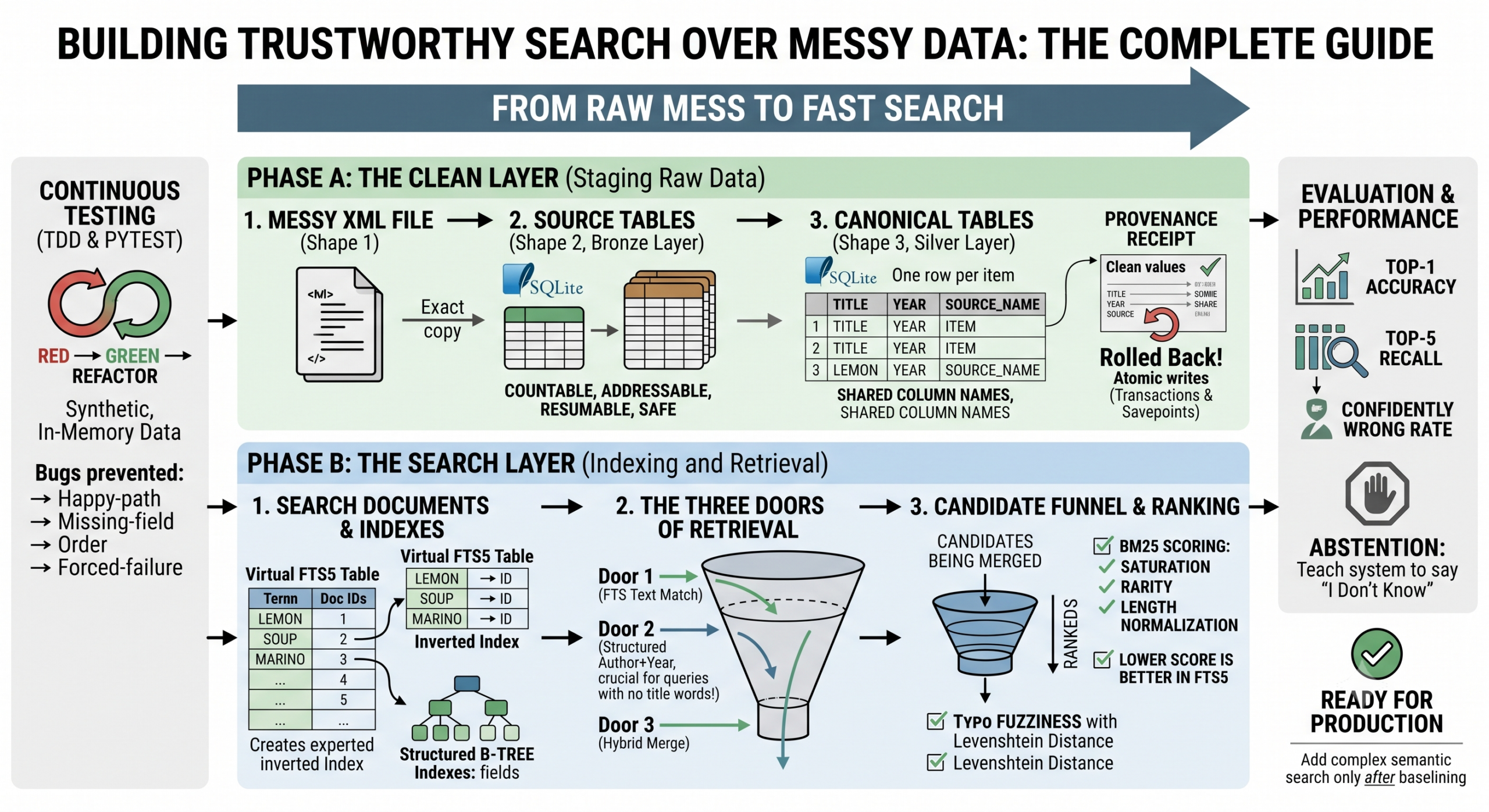
From a 5 GB Mess to Fast Search: The Clean Layer and the Search Layer
A plain-English deep dive into canonical mapping, indexing, retrieval channels, and the tests that keep them honest — by ingoampt.
Imagine you inherit a giant file. It is an XML export of thousands of recipes from an old cooking website your grandmother loved. There are also other piles: a spreadsheet of magazine clippings, a folder of scanned index cards. Every source names its fields differently. One day you want to type something vague — “grandma’s lemon soup thing from 2019” — and get the exact recipe back. This article shows you, step by step, how to get there.
You reach reliable search in two big phases. Phase A (the clean layer) turns preserved raw records into one shared tidy shape. Phase B (the search layer) makes that tidy shape fast to search through several retrieval channels. Automated tests sit at every step because you cannot eyeball five million rows, and a test re-checks your work forever. Do these in order and a vague query finds the right recipe; skip the clean layer and search silently fails.
1. One recipe, three shapes
We follow a single recipe through three shapes. Watch the same facts move from a tangled text file, into an exact copy inside a database, and finally into a tidy shape you can search. A shape here just means “the layout the data sits in.”
Shape 1 — the original XML file
XML (eXtensible Markup Language) is a way of writing data as nested tags, like labelled boxes inside boxes. Here is one recipe as it sits in the giant export:
<recipe id="soups/lemon/Rosa19" updated="2019-05-10">
  <author>Rosa Marino</author>
  <author>Mira Costa</author>
  <title>Lemon Soup with Herbs</title>
  <cookbook>Nonna's Kitchen</cookbook>
  <year>2019</year>
  <link type="scan">scans/soups/Rosa19.jpg</link>
</recipe>
This looks fine for one recipe. But the real file holds thousands of them, and the whole thing is about 5 gigabytes of text — roughly the size of a thousand thick paperback books glued into one scroll. You cannot ask it “how many soups do I have?” without reading the entire scroll top to bottom. There are no rows, no columns, no totals. The data is trapped inside nested text.
Shape 2 — source tables: an exact, faithful copy
The first real move is to copy the XML into a database without changing a single value. We use SQLite: a small, reliable database engine that stores an entire database in a single file on disk, needs no separate server, and ships built into Python as the sqlite3 module. That module includes FTS5 full-text search support in every standard Python 3.10+ distribution, so nothing extra needs installing. Because SQLite is one file, the raw copy and the clean copy can live side by side and nothing ever leaves SQL.
We store the copy in three tables. This is a faithful mirror: it keeps values, field names, order, and attributes exactly.
Table source_records — one row per top-level item.
| row_id | key | type |
|---|---|---|
| 1 | soups/lemon/Rosa19 | recipe |
Table source_field_occurrences — one row per field, in original order. Note six rows for this one recipe.
| field_id | row_id | field_name | text | position |
|---|---|---|---|---|
| 4821 | 1 | author | Rosa Marino | 1 |
| 4822 | 1 | author | Mira Costa | 2 |
| 4823 | 1 | title | Lemon Soup with Herbs | 3 |
| 4824 | 1 | cookbook | Nonna’s Kitchen | 4 |
| 4825 | 1 | year | 2019 | 5 |
| 4826 | 1 | link | scans/soups/Rosa19.jpg | 6 |
Table source_field_attributes — the little labels attached to a field, such as type="scan" on the link.
| field_id | attribute_name | value |
|---|---|---|
| 4821 | — | — |
| 4826 | type | scan |
This copy preserves everything — values, names, order, and attributes. From these three tables you could rebuild the original XML byte for byte. That faithfulness is the whole point of this stage. It mirrors the modern data-engineering “bronze” (raw) layer, whose principle is simple: capture everything, transform nothing.
Shape 3 — canonical tables: the tidy shape
Now the interesting work: reshape the faithful copy into a clean, shared layout — one row per item, with the same column names for the same ideas. This is the “silver” (cleaned) layer.
clean_recipes
| row_id | type | title | year | source_name |
|---|---|---|---|---|
| 1 | recipe | Lemon Soup with Herbs | 2019 | Nonna’s Kitchen |
clean_contributors — order preserved: contributor 1 stays contributor 1.
| row_id | role | position | name |
|---|---|---|---|
| 1 | author | 1 | Rosa Marino |
| 1 | author | 2 | Mira Costa |
clean_links
| row_id | kind | value | type |
|---|---|---|---|
| 1 | image | scans/soups/Rosa19.jpg | scan |
clean_identifiers
| row_id | scheme | value |
|---|---|---|
| 1 | source_key | soups/lemon/Rosa19 |
clean_provenance — the receipt: which clean value came from which source field, and which rule produced it.
| clean_target | from source field_id | rule |
|---|---|---|
| clean_recipes.title | 4823 | direct_copy |
| clean_recipes.year | 4825 | parse_year |
| clean_recipes.source_name | 4824 | map_source_name |
| clean_contributors[1] | 4821 | direct_copy |
| clean_links.value | 4826 | direct_copy |
2. Why copy XML into SQL at all?
A fair question: why not read the XML and write the clean tables directly? Because the raw text file is a terrible place to work. Here are five concrete reasons, each with an example.
(a) You cannot reliably count or audit a 5 GB text file
Plain English: a giant scroll of text gives you no totals.
AnalogyCounting recipes in the XML is like counting every red car in a city by walking every street once. Counting them in SQL is like asking the parking office for the number.
Example: in SQL you write SELECT type, COUNT(*) FROM source_records GROUP BY type; and instantly learn you have 8,412 recipes, 210 menus, and 17 datasets. In raw XML you would have to stream all 5 GB and hand-write a counter, and any mistake gives a silently wrong total.
(b) A multi-hour job must be restartable
Plain English: long jobs crash; you need to resume, not restart.
AnalogySQL rows are like numbered pages in a ledger — if you stop at page 3,000 you carry on from 3,001. An XML stream is like reading a scroll with no page numbers; a crash sends you back to the top.
Example: your transform runs for three hours and the laptop sleeps at hour two. With row_id values and a checkpoint, you resume at row_id 5,001. With raw XML there is no resume point.
(c) Provenance needs stable addresses
Plain English: to prove where a clean value came from, each source value needs a permanent address.
AnalogyAn address like field_id 4824 is a house number. You can always point back to it. A phrase buried in nested XML is like saying “the third house-ish thing on the left, I think.”
Example: the clean source_name “Nonna’s Kitchen” records that it came from field_id 4824 via rule map_source_name. XML has no equivalent stable ID.
(d) Re-reading 5 GB for every fix is impossibly slow
Plain English: during development you touch the data thousands of times.
AnalogyFetching one SQL row is like flipping to one page. Re-parsing the XML each time is like re-reading the whole scroll to check one sentence.
Example: a test that checks one recipe fetches WHERE row_id = 1 in well under a millisecond. Re-streaming the XML for that same check could take minutes — multiplied by every test run, that is hours wasted per day.
(e) Doing the hardest step with no safety net is reckless
Plain English: the reshape is the risky part; do it against a stable, inspectable copy.
WarningIf you transform straight off a giant text file, a single bug in hour two can corrupt the whole run and you may not notice until the end. With the raw copy safe in SQL, you rebuild the clean layer as many times as you like, risk-free.
| Property | XML file | Source tables | Canonical tables |
|---|---|---|---|
| Faithful to original | Yes (it is the original) | Yes (exact copy) | No (reshaped on purpose) |
| Countable | No | Yes | Yes |
| Resumable | No | Yes | Yes |
| Addressable (stable IDs) | No | Yes | Yes |
| Searchable | No | No | Yes |
3. Why a second set of tables, not cleaning in place?
Plain English: keep the raw copy read-only forever; build the clean copy beside it.
Analogy — the museum-original ruleThe source tables are the museum original. You never paint over a museum painting to “fix” it. You make a study copy and work on that. If your clean copy is wrong, you throw it away and rebuild from the untouched original — as many times as you need.
Both sets of tables live in the same SQLite file. Nothing is exported, nothing leaves SQL. This is exactly the raw-then-cleaned staging pattern used across modern data engineering: because all data sits in immutable raw tables, you can always recreate downstream tables, add columns, rebuild, or recover when the cleaning logic changes.
Cleaning in place destroys your only faithful record. A second set of tables means a bug in the transform is never fatal — the truth is still sitting untouched next door.
4. Why the source tables cannot be indexed usefully
This is the insight the whole project turns on. In the source shape, there is no “title” column. The word “title” is a value sitting in a field_name cell. The text column holds titles, names, years, and links all mixed together.
There is a second problem: different item types put the same idea under different field names. A soup uses cookbook. A website recipe uses website_name. A magazine clipping uses magazine. A single query over the raw tables cannot find them all, because they do not share a name. Only after the clean layer maps all three into one source_name column can a single index and a single query serve every type.
The clean layer makes indexing possible. The index makes search fast. You need both, in that order.
5. Phase A in full detail: the clean layer
The clean layer has to make a series of careful decisions. Here is everything it decides.
Type mapping
Each raw item has a type, and each type maps to a clean shape. Different types have slightly different rules, so you add support for them one or two at a time — never all at once.
| Raw item | Maps to | Note |
|---|---|---|
| Main dish | recipe | the common case |
| Drink | recipe | same clean shape |
| Chapter of a baking book | recipe linked to a parent | keeps a pointer to the book |
| Menu | container | holds other items |
| Data entry | dataset | tabular source, not a recipe |
Field-by-field mapping
This table shows which source field becomes which clean column — and how one clean column, source_name, is fed by three different raw names depending on type.
| Source field | Clean column | Depends on type? |
|---|---|---|
| title | clean_recipes.title | no |
| year | clean_recipes.year | no |
| author | clean_contributors.name | no |
| cookbook (soup) | clean_recipes.source_name | yes |
| website_name (website recipe) | clean_recipes.source_name | yes |
| magazine (clipping) | clean_recipes.source_name | yes |
The never-guess rule
Plain English: if a value is missing, leave it missing. Do not invent.
In databases, NULL means “no value is recorded.” That is different from an empty string "", from the number 0, and from the word "unknown". Each of the last three is a claim; NULL is honest silence.
| You write | It means | Correct for a missing year? |
|---|---|---|
| NULL | we do not know the year | Yes — the honest choice |
| “” | the year is the empty text | No — invents a blank value |
| 0 | the year is zero | No — invents a wrong number |
| “unknown” | the year is the word unknown | No — pollutes a number column |
WarningNever copy a value from a neighbouring row to fill a gap. A missing author is not “probably the same as the last one.” Missing stays NULL.
Preserving order and exact text
Order carries meaning: the first author may be the lead cook. So contributor 1 stays contributor 1, tracked by the position column. And exact text is sacred:
ExampleThe link is stored as scans/soups/Rosa19.jpg. It is tempting to “helpfully” rewrite it as https://example.com/scans/soups/Rosa19.jpg. Do not. You would be inventing a web address that may not exist. Copy the value exactly as found.
Provenance receipts
Every clean value records where it came from and how. Provenance is the origin of a specific data point: which source it came from and what rule produced it. (Its cousin, lineage, is the broader journey of data across systems over time.) This is what the clean_provenance table stores.
Atomic writing: transactions and savepoints
When you write one clean recipe, you write several rows across several tables. If the program crashes halfway, you must not leave a half-written recipe. Databases solve this with transactions. A transaction is a group of writes that all succeed together or all get undone together — the “A” (atomicity) in ACID, the four reliability promises databases make (Atomicity, Consistency, Isolation, Durability).
SQLite also offers SAVEPOINT: a marker inside a transaction you can roll back to without abandoning everything before it. You set a savepoint per item; if that item fails, you ROLLBACK TO the savepoint and the half-written rows vanish, while the good items before it stay.
Underneath, SQLite protects the file itself with a rollback journal. As the official documentation explains, if power fails mid-write, on the next open recovery makes it appear either as if no changes were made or as if the complete set of changes was made — never a half-state.
Reconciliation at the end
When the transform finishes, per-type counts must match the numbers you measured at the very start. And you must check counts per type, not just the grand total — because a grand total can hide a compensating error.
Worked exampleYou started with 8,412 recipes and 210 menus (total 8,622). After the run you have 8,312 recipes and 310 menus. The grand total is still 8,622 — looks fine! But 100 recipes were wrongly mapped as menus. Only a per-type check catches this: recipes are short by 100, menus are over by 100.
6. Why tests — and what each one catches
You might think you can just look at the output in the terminal. You cannot. You can eyeball 5 items; you cannot eyeball 5 million. And a manual check is a one-time thing — it says nothing about tomorrow, after someone edits the code. A test re-checks your rules forever, automatically, every time anyone changes anything.
Each test type maps to a specific bug
| Test | The exact bug it prevents |
|---|---|
| Happy-path test | Wrong values written for a normal, complete item |
| Missing-field test | Junk empty rows written when a field is absent |
| Empty-field test | Same, but for blank strings "" that sneak past |
| Order test | Contributors returned in the wrong order |
| Exact-text test | Values silently “helpfully” rewritten (the link case) |
| Unknown-type guard test | Unsupported items silently dropped or half-mapped |
| Duplicate-mapping test | The same item written twice |
| Snapshot before/after test | The raw source accidentally modified |
| Row-count-across-all-tables test | Rows written where they should not exist |
| Forced-failure test | Half-written items surviving a simulated crash |
The forced-failure test is worth a word: you deliberately break a write partway (for example with a database trigger that raises an error on the second table), then assert that nothing from that item remains. That proves your transaction/savepoint logic actually rolls back — you tested the safety net instead of hoping.
Test-driven development: red, green, refactor
Test-driven development (TDD) flips the usual order: you write the test first, watch it fail, then write just enough code to make it pass. Kent Beck, who formalised TDD in his 2002 book Test-Driven Development: By Example (Addison-Wesley), states two simple rules: “Write new code only if an automated test has failed” and “Eliminate duplication.” From these, he says, follows the mantra Red → Green → Refactor: “Red — write a little test that doesn’t work, perhaps doesn’t even compile at first. Green — make the test work quickly, committing whatever sins necessary in the process. Refactor — eliminate all the duplication created in just getting the test to work.”
Why a pre-existing pass is suspiciousIf you write a test for a feature that does not exist yet and it passes immediately, be worried. Either the behaviour already exists (so you did not need to write it), or — far more likely — your test is not actually testing what you think. Watching it fail first proves the test can fail, so a later pass means something real.
Reading pytest output
pytest is Python’s most popular test runner. It discovers files named test_*.py and functions named test_* automatically. A run looks like this:
$ pytest
==================== test session starts ====================
platform linux -- Python 3.12, pytest-8.3.3
collected 65 items / 57 deselected / 8 selected

tests/test_clean.py ...FF.F                            [100%]

========================= FAILURES ==========================
... assertion details ...
========= 3 failed, 5 passed, 57 deselected in 0.42s ========
Line by line: collected 65 items — pytest found 65 tests. 57 deselected — you used a filter (for example -k clean) so 57 tests were set aside and not run this time; deselected is not a failure, it just means “found but not chosen.” 8 selected — the 8 that matched your filter actually ran. The dots and letters show each result: . is a pass, F is a failure. The final line totals it: 3 failed, 5 passed, 57 deselected. Three tests are telling you something is wrong; fix the code until they turn into dots.
Synthetic test data
You do not test against the real 5 GB file. You use synthetic data: tiny, made-up items — a couple of fake recipes — loaded into a throwaway in-memory SQLite database (sqlite3.connect(":memory:")). Fake and small buys three things:
- Speed: an in-memory database with two rows runs in milliseconds, so the whole suite finishes in under a second.
- Repeatability: the same tiny input gives the same result every run, on every machine.
- Safety: a throwaway database cannot damage your real data, no matter what the test does.
7. Phase B in full detail: the search layer
Now the clean layer exists, we make it fast to search. This is where a vague query turns into the right recipe.
Building search documents
For each recipe we build one combined searchable text — a search document — by joining the useful fields: title + contributors + source name + year. For our recipe that string is:
Lemon Soup with Herbs Rosa Marino Mira Costa Nonna's Kitchen 2019One blob per recipe means the search engine has a single place to look.
Exact identifier lookup — instant, highest confidence
If the query contains a known key (like soups/lemon/Rosa19) or a scheme-based code (an ISBN-style identifier), you skip search entirely and look it up directly. This is the fastest, most trustworthy channel: an exact match is not a guess.
What an index actually is
AnalogyAn index is the index at the back of a book. Without it, finding every mention of “lemon” means reading every page (a full scan). With it, you jump straight to the listed pages.
Technically, a database index is usually a B-tree: a balanced, sorted tree of values with pointers to rows. Instead of checking every row one by one (which costs time proportional to the number of rows), the database descends a shallow tree in a handful of steps. On a table of 100 million rows, that is roughly the difference between 100 million comparisons and about 27 — an enormous reduction in work. Real-world indexes reach any row in four to six steps, because each tree node holds hundreds of entries, which keeps the tree shallow.
Full-text search with FTS5
SQLite ships a full-text search engine called FTS5. You create a virtual table and it builds an inverted index — a map from each word (token) to the list of documents that contain it, so “lemon” points straight to every recipe mentioning lemon. You query it with the MATCH operator:
CREATE VIRTUAL TABLE recipes_fts USING fts5(search_document);

SELECT rowid FROM recipes_fts
WHERE recipes_fts MATCH 'lemon soup'
ORDER BY rank;
Per SQLite’s official documentation, FTS5 has been included as part of the SQLite amalgamation since version 3.9.0 (2015-10-14). It tokenizes text on insert and understands phrase queries, prefix queries, and boolean operators (AND, OR, NOT).
BM25 ranking, without heavy maths
When several recipes match, which comes first? FTS5 ranks with BM25, a probabilistic ranking function developed by Stephen Robertson and Karen Spärck Jones out of 1970s–1980s information-retrieval research (the name comes from the 25th “Best Match” experiment in that programme). Three intuitions:
- Term frequency with diminishing returns: a recipe that says “lemon” five times is more relevant than one that says it once — but not five times as relevant. After a few mentions, extra ones barely move the score. This flattening is called saturation.
- Rare words count more: a rare surname like “Marino” is a stronger signal than a common word like “the”. BM25 weights rare terms up and common terms down. This is IDF, inverse document frequency.
- Document-length normalisation: a long document naturally contains more words, so BM25 discounts length to stop long recipes from winning just for being wordy.
A gotcha worth knowingPer the official SQLite FTS5 documentation, the built-in bm25() function returns a value where “the better the match, the numerically smaller the value returned.” FTS5 multiplies the standard result by −1 so that better matches get smaller (more negative) numbers; therefore the default ascending ORDER BY rank returns the best matches first. The tuning constants k1 and b are hard-coded at 1.2 and 0.75 respectively. Beginners expect “higher is better” and get it backwards — in FTS5, lower is better.
The three doors
This is the part most home-grown search systems get wrong. Different messy queries need different retrieval channels — different “doors” into the data. A system with only text search silently fails on some perfectly reasonable queries.
| Door | Query looks like | Channel used | Why text-only search fails it |
|---|---|---|---|
| 1 | Lemon Soup with Herbs | FTS5 text search + BM25 | — |
| 2 | Marino 2019 | structured author + year lookup | no title words exist to match |
| 3 | Rosa’s lemon soup from 2019 | author lookup + topic text search, merged | partly works, but misses without the author channel |
A system with only text search returns nothing for “Marino 2019” and looks broken. Door 2 — matching the name against clean_contributors and the year against clean_recipes.year — is the only door that opens that query.
Short compact codes
Some queries contain squashed venue-and-year tokens. Invent the recipe-world equivalent: a user types nonna19, meaning the cookbook “Nonna’s Kitchen” plus 2019. A small hand-written lookup table can expand nonna → “Nonna’s Kitchen” and split off 19 → 2019.
WarningThese expansions must produce candidates, not certainties. “nonna” might mean a different cookbook in another user’s archive. Feed the guess into the candidate pool; never treat it as a confirmed answer.
Merging candidates into one shortlist
Each channel proposes candidates. You merge them into one candidate set, then rank. Picture a funnel: millions of rows narrow to a handful of strong candidates, then to one confident answer.
Fuzzy matching for typos
People misspell things. Levenshtein distance (edit distance) counts the minimum number of single-character edits — insertions, deletions, or substitutions — needed to turn one word into another. “lemmon” → “lemon” is distance 1 (delete one m); the classic textbook example “kitten” → “sitting” is distance 3. A small edit distance means “probably a typo of,” so you can rescue a near-miss query. Note its blind spot: it compares letters, not meaning, so “big” and “large” are far apart despite meaning the same thing.
Embeddings come later — and only if measured
You may have heard of semantic search with embeddings (turning text into meaning-vectors so “soup” and “broth” sit near each other). Build the simple lexical baseline (exact lookup + FTS5 + BM25) first. Two reasons:
- You need a baseline to measure against. Without it you cannot prove embeddings actually helped.
- Meaning-based search adds nothing when a query is just a surname and a year. “Marino 2019” has no meaning to capture — it needs the structured Door 2, not a fancy vector.
Key idea
Add complexity only when measurement proves it earns its place. Lexical retrieval (BM25) remains a strong, cheap baseline; it is precise on exact terms and rare names, and it often acts as the guardrail that stops meaning-based search from drifting. Layer semantics on top later if the numbers justify it.
Evaluation: measure, especially “confidently wrong”
Test the search against a known list of messy queries whose right answers you already know. Measure:
- Top-1 accuracy: how often the very first result is correct.
- Top-5 recall: how often the correct recipe appears somewhere in the top five.
- Confidently wrong rate: how often the system returned a wrong answer while acting sure. This is the number that matters most.
Abstention beats a confident lie
Teach the system to say “no confident match” when its best candidate is weak. A returned “I’m not sure” is far better than a confident wrong recipe, because a confident wrong answer quietly destroys the user’s trust. Track the abstention rate alongside accuracy, and treat a correct abstention as a success, not a miss.
8. The whole journey, in order
| Phase | What you do | What it produces |
|---|---|---|
| Raw capture | Copy XML into SQLite exactly | Source tables — a faithful, countable, addressable mirror |
| Clean (Phase A) | Map types and fields into one shared shape, with provenance | Canonical tables — one row per item, shared columns |
| Index | Build search documents, B-tree indexes, and the FTS5 inverted index | Fast lookup structures |
| Retrieve (Phase B) | Run exact lookup + text + author/year, merge candidates | A ranked shortlist per query |
| Rank | Order candidates with BM25 (lower is better) | A best answer, or an honest abstention |
| Measure | Score top-1, top-5, and confidently-wrong on known queries | Evidence for what to improve next |
9. Reusable checklist
- ☐ Copy raw data into SQL exactly before changing anything.
- ☐ Keep the raw tables read-only; build clean tables beside them in the same file.
- ☐ Give every source field a stable ID for provenance.
- ☐ Map types and fields deliberately; add one type at a time.
- ☐ Never guess — missing stays NULL, and exact text stays exact.
- ☐ Preserve order with an explicit position column.
- ☐ Write each item atomically with a transaction and a savepoint.
- ☐ Reconcile per-type counts against the start; never trust the grand total alone.
- ☐ Write a failing test first; watch it go red, then green.
- ☐ Test on tiny synthetic data in an in-memory database.
- ☐ Build search documents; index them; expose exact, text, and author/year doors.
- ☐ Rank with BM25 (remember: lower is better in FTS5).
- ☐ Prefer abstention over a confident wrong answer.
- ☐ Add embeddings only after measurement proves they help.
10. FAQ
- Do I really need SQLite specifically?
- No — any SQL database works. SQLite is convenient because the whole database is one file, it needs no server, it ships inside Python’s standard library as
sqlite3, and it includes FTS5 for full-text search out of the box. - Why keep the raw copy if it wastes disk space?
- Because it is your only faithful record. When a cleaning rule turns out wrong, you rebuild the clean layer from the untouched raw copy instead of re-parsing 5 GB or, worse, having lost the original.
- Why is a missing value NULL and not 0 or “unknown”?
- NULL means “we do not know.” 0, “”, and “unknown” are all claims about the value that you cannot back up. Inventing them pollutes your data and produces wrong answers later.
- What does “deselected” mean in pytest?
- It means those tests were found but not chosen to run this time, usually because of a filter like
-k. It is not a failure — just “set aside for now.” - Why write the test before the code?
- So you can watch it fail for the right reason. A test that passes before the feature exists is not testing what you think. Failing first proves the test works. This is the heart of Kent Beck’s rule: write new code only if an automated test has failed.
- Why is a lower BM25 score better in SQLite?
- FTS5 multiplies the standard BM25 result by −1 so that better matches get smaller numbers, letting the default ascending
ORDER BY rankreturn the best matches first. - What’s the single most common search-system mistake?
- Building only text search. Queries like “Marino 2019” have no title words, so text search returns nothing and the system looks broken. You need an author-plus-year door too.
- When should I add semantic/embedding search?
- Only after your lexical baseline is measured, and only if embeddings measurably beat it. For name-and-year queries, embeddings add nothing.
- What’s the difference between provenance and lineage?
- Provenance is the origin of a specific value (where it came from and what rule made it). Lineage is the broader journey of data across systems over time. This article’s receipts are provenance.
- How small should synthetic test data be?
- As small as possible — one or two hand-made items. Small means fast, repeatable, and safe, and it still exercises every rule you care about.
INFOGRAPHIC GUIDE:
FROM MESSY DATA TO TRUSTWORTHY SEARCH
Based on the architecture by ingoampt: Clean Layer, Search Layer, and Test-Driven Reliability.
1. THE MACRO PIPELINE AT A GLANCE
┌─────────────────┐     ┌─────────────────┐     ┌─────────────────┐
│     SHAPE 1     │     │     SHAPE 2     │     │     SHAPE 3     │
│   Messy XML     │ ──► │  Source Tables  │ ──► │ Canonical Tables│
│ (Raw text file) │     │ (Bronze / Raw)  │     │ (Silver / Clean)│
└─────────────────┘     └─────────────────┘     └─────────────────┘
                                                         │
                                                         ▼
┌─────────────────┐     ┌─────────────────┐     ┌─────────────────┐
│ Rerank & Score  │     │ 3-Door Candidate│     │ Virtual FTS5 &  │
│ (BM25 / Abstain)│ ◄── │    Retrieval    │ ◄── │ B-Tree Indexes  │
└─────────────────┘     └─────────────────┘     └─────────────────┘
2. PHASE A: THE CLEAN LAYER (DATA EVOLUTION)
Step 1: The Three Data Shapes
SHAPE 1: Original XML File (~5 GB) ┌────────────────────────────────────────────────────────┐ ││ │ Rosa Marino │ │Lemon Soup with Herbs │ │Nonna's Kitchen │ │2019 │ └────────────────────────────────────────────────────────┘ ❌ Cannot query easily ❌ Uncountable ❌ Unresumable │ Copy directly without changing a single byte ▼ SHAPE 2: Source Tables in SQLite (Bronze Layer) ┌────────────────────────────────────────────────────────────────────────┐ │ source_records: row_id: 1 | key: soups/lemon/Rosa19 │ │ source_field_occurrences: field_id: 4821 | author | Rosa Marino │ │ field_id: 4823 | title | Lemon Soup... │ │ field_id: 4824 | cookbook | Nonna's Kitchen │ │ field_id: 4825 | year | 2019 │ └────────────────────────────────────────────────────────────────────────┘ ✓ Faithful mirror ✓ Countable & audit-ready ✓ Stable field_ids │ Transform & map clean rules ▼ SHAPE 3: Canonical Tables in SQLite (Silver Layer) ┌────────────────────────────────────────────────────────────────────────┐ │ clean_recipes: row_id: 1 | title: Lemon Soup... | year: 2019 │ │ clean_contributors: row_id: 1 | role: author | position: 1 | Rosa... │ │ clean_provenance: clean_target: title | source_field_id: 4823 │ └────────────────────────────────────────────────────────────────────────┘ ✓ One row per item ✓ Shared standard columns ✓ Ready for indexing
Why Copy XML to SQL First?
| Feature | Raw XML File | Source Tables (SQLite) |
|---|---|---|
| Auditing & Counts | Full 5 GB scan needed | Instant SQL COUNT(*) queries |
| Crash Recovery | Restarts from byte 0 | Resumes at row_id checkpoint |
| Provenance | Loose string offsets | Permanent, stable field_id addresses |
| Test Speed | Slow streaming (minutes) | Sub-millisecond lookup per test |
| Safety Net | High risk of file corruption | Read-only raw copy; destroyable clean tables |
Core Clean Layer Rules
 1. TYPE MAPPING         ──► Map recipes, menus, datasets one by one.
 2. UNIFIED COLUMNS      ──► Map "cookbook", "website", & "magazine" all
                             into a single "source_name" column.
 3. NEVER GUESS          ──► Missing data stays NULL.
                             Never put "" or 0 or "unknown".
 4. EXACT COPY           ──► Keep links & strings strictly intact.
                             Never rewrite URL structures.
 5. PROVENANCE RECEIPT   ──► Store receipt in `clean_provenance`:
                             (clean_col ◄── source_field_id + rule_name)
 6. PER-TYPE AUDITING    ──► Match raw vs. clean counts *per type*,
                             never rely on grand totals alone.
Transaction & Savepoint Safety
Attempting to write Recipe #2:
┌────────────────────────────────────────────────────────────────┐
│ 1. SET SAVEPOINT sp2;                                          │
│ 2. INSERT INTO clean_recipes (...)  ──► SUCCESS                │
│ 3. INSERT INTO clean_contributors   ──► CRASH! (Database Error) │
│ 4. ROLLBACK TO sp2;                                            │
└────────────────────────────────────────────────────────────────┘
                               │
                               ▼
┌────────────────────────────────────────────────────────────────┐
│ RESULT: Half-written Recipe #2 vanishes completely.             │
│ Recipe #1 remains perfectly safe and intact.                   │
└────────────────────────────────────────────────────────────────┘
3. TESTING ENGINE & TDD FLOW
The Red-Green-Refactor Loop
  ┌───────────────────────────────────────────────────────────┐
  │ 🔴 RED: Write a failing unit test first.                  │
  │    (Proves the test works and detects missing features)   │
  └─────────────────────────────┬─────────────────────────────┘
                                │
                                ▼
  ┌───────────────────────────────────────────────────────────┐
  │ 🟢 GREEN: Write minimum production code to pass the test. │
  └─────────────────────────────┬─────────────────────────────┘
                                │
                                ▼
  ┌───────────────────────────────────────────────────────────┐
  │ 🔵 REFACTOR: Tidy code and eliminate duplication.          │
  └───────────────────────────────────────────────────────────┘
Anatomy of pytest Output
$ pytest -k clean

collected 65 items / 57 deselected / 8 selected
tests/test_clean.py ...FF.F                                [100%]

============================= FAILURES =============================
...

 57 deselected ──► Ignored by filter (-k)
 3 passed (.)  ──► Passed successfully
 3 failed (F)  ──► Bugs detected, code needs fixing!
4. PHASE B: THE SEARCH LAYER
Structural vs. Full-Text Indexes
  B-Tree Index (Structured Columns)       Inverted Index (FTS5 Text Search)
┌───────────────────────────────────┐   ┌───────────────────────────────────┐
│   Year Tree    ──► Row Pointers   │   │  Term        ──► Document IDs    │
│   [2018]       ──► Row 14, 88     │   │  "lemon"     ──► Doc 1, Doc 42   │
│   [2019]       ──► Row 1, 9, 102  │   │  "soup"      ──► Doc 1, Doc 15   │
└───────────────────────────────────┘   └───────────────────────────────────┘
   Allows instant exact filtering          Allows instant phrase & term matching
The 3 Doors of Search Retrieval
                      USER QUERY ATTEMPT
                              │
     ┌────────────────────────┼────────────────────────┐
     ▼                        ▼                        ▼
┌─────────┐              ┌─────────┐              ┌─────────┐
│ DOOR 1  │              │ DOOR 2  │              │ DOOR 3  │
└────┬────┘              └────┬────┘              └────┬────┘
     │                        │                        │
  Text Query               Name + Year             Hybrid Query
  "Lemon Soup"            "Marino 2019"         "Rosa Lemon 2019"
     │                        │                        │
     ▼                        ▼                        ▼
FTS5 Full-Text           Structured SQL             Merged FTS5 +
Search + BM25           Author + Year          Structured Lookup
                          Lookup
     │                        │                        │
     └────────────────────────┼────────────────────────┘
                              │
                              ▼
                     CANDIDATE FUNNEL
⚠️ Critical Insight:
Text search fails completely on Door 2 (“Marino 2019”) because the query contains zero title words. You must provide a structured lookup door.
Ranking Mechanics: SQLite FTS5 & BM25
BM25 scores search matches using three core ideas:
1. Term Frequency (TF)       ──► More keyword occurrences = higher relevance
                                  (with diminishing returns/saturation).
2. Inverse Doc Frequency(IDF)──► Rare words ("Marino") weigh significantly
                                  more than common words ("Soup").
3. Document Length Norm      ──► Penalizes longer text blobs so they don't
                                  win just by having more words.
 ⚠️ SQLITE FTS5 GOTCHA:
 In SQLite FTS5, BM25 scores are multiplied by -1.
 LOWER / MORE NEGATIVE NUMBERS = BETTER MATCH!

 Correct Query: SELECT rowid FROM recipes_fts
                WHERE search_document MATCH 'lemon'
                ORDER BY rank;  -- Ascending order gives best results!
5. REFINEMENT, MEASUREMENT & HYBRID CANDIDATE FUNNEL
           [ All Raw Database Records (~Millions) ]
                          │
                          ▼  (Retrieval via 3 Doors)
      [ Candidate Pool: Merged Exact + FTS + Structured ]
                          │
                          ▼  (Typo Resilience via Levenshtein Distance)
            [ Filtered & Normalized Candidates ]
                          │
                          ▼  (BM25 Scoring & Ranking)
             [ Sorted Shortlist of Results ]
                          │
              ┌───────────┴───────────┐
              ▼                       ▼
    Score >= Threshold       Score < Threshold
              │                       │
              ▼                       ▼
    [ Confident Top-1 ]     [ Abstain: "No Confident Match" ]
6. MASTER IMPLEMENTATION CHECKLIST
- ☐ 1. Exact Raw Capture: Copy source XML into SQLite tables without changing values.
- ☐ 2. Read-Only Raw Layer: Never modify raw source tables. Build clean tables beside them.
- ☐ 3. Stable Provenance: Assign a permanent
field_idto every raw field occurrence. - ☐ 4. Never Guess: Leave unknown fields as
NULLinstead of empty strings or zeroes. - ☐ 5. Atomic Writes: Enclose item transformations in transactions and
SAVEPOINTs. - ☐ 6. Per-Type Auditing: Check post-cleaning row counts per item type against original counts.
- ☐ 7. TDD Approach: Write failing tests against synthetic in-memory databases before writing code.
- ☐ 8. Multichannel Retrieval: Build distinct retrieval paths for FTS5, Structured Metadata, and Hybrids.
- ☐ 9. BM25 Ranking: Sort FTS5 search by ascending
rank(ORDER BY rank). - ☐ 10. Safe Abstention: Teach the search engine to abstain when candidate match scores are low.