INGOAMPT · Learn
How Search Engines Find Anything in Milliseconds: 14 Data & Search Terms Explained for Beginners
Every search box you have ever typed into — a library catalog, an online shop, a music app — sits on top of two invisible stages: a data pipeline that loads millions of records safely, and an information retrieval engine that finds the right one in milliseconds. This guide explains every core term of both stages with drawings, tables, and real code, assuming zero background.
- Part 1 — Getting data in safely: Streaming · Parsing · DTD & entities · Schema & ingestion · Immutability · Reconciliation · Knowing your numbers
- Part 2 — Finding things fast: Inverted index · BM25 · Candidates → reranking · Edit distance & trigrams · Top-k accuracy & MRR · Precision vs recall · Baseline
The running example. Throughout this article, imagine you are building a search engine for a giant library catalog: a single 5 GB file containing about 12 million book and article records, from which you must answer messy human queries like “atention is all yu need” — and still return the right paper. Everything below is a tool for exactly that job.
Part 1 · Getting Data In Safely (The Pipeline Phase)
Before you can search anything, you must move millions of raw records from a downloaded file into your own database — without corrupting a single one. These seven terms describe that journey.
1. Streaming
Memory managementSuppose your catalog file is 5 GB of text and your laptop has 8 GB of RAM. If your program loads the entire file into memory, plus the parsed objects it builds from it (which typically take 3–5× more space than the raw text), you crash. Streaming means your program holds only one record in memory at any moment: read it, process it, throw it away, read the next. Memory use stays flat — “bounded” — no matter how big the file is.
In Python, the difference is one function call:
<span class="c"># ❌ Loads all 5 GB into RAM at once</span>
data = open("catalog.xml").read()

<span class="c"># ✅ Streams: yields one record at a time, constant memory</span>
<span class="k">for</span> event, element <span class="k">in</span> ET.iterparse("catalog.xml"):
    process(element)
element.clear() <span class="c"># free the record we just handled</span>2. Parsing
Raw text → structured objectsA file on disk is just characters. The text <title>Attention Is All You Need</title> is, to the computer, 45 meaningless bytes. Parsing is the act of recognizing the grammar in those bytes and producing a validated object with named fields. Here is one raw record and the object a parser builds from it:
<span class="c"><!-- BEFORE: raw XML text in the file --></span>
<article key=<span class="k">"journals/ml/Vaswani17"</span>>
  <author>Ashish Vaswani</author>
  <title>Attention Is All You Need</title>
  <year>2017</year>
</article>

<span class="c"># AFTER: a validated Python object</span>
Record(
    key    = <span class="k">"journals/ml/Vaswani17"</span>,
    authors= [<span class="k">"Ashish Vaswani"</span>],
    title  = <span class="k">"Attention Is All You Need"</span>,
    year   = 2017          <span class="c"># note: now a NUMBER, not text</span>
)Parsing is also your first quality gate. If a record says <year>20I7</year> (a typo with the letter I), a good parser raises an error at the door instead of quietly storing corrupt data.
3. DTD & Entities
XML grammaré is the nickname for é.DTD stands for Document Type Definition. Big XML datasets ship with one so every program on Earth agrees on the grammar. A tiny DTD for our catalog might say:
<span class="c"><!-- catalog.dtd — the rulebook --></span>
<!ELEMENT article (author+, title, year)> <span class="c"><!-- an article = 1+ authors, then title, then year --></span>
<!ELEMENT author (#PCDATA)> <span class="c"><!-- author contains plain text --></span>
<!ENTITY eacute "é"> <span class="c"><!-- define nickname: eacute → character 233 = é --></span>Why do entities exist? Old files could only safely store basic ASCII characters (A–Z, 0–9). Accented names had to be spelled with nicknames. Your parser must translate them, or names get silently mangled:
| Written in the file | Entity means | What the reader should see |
|---|---|---|
Renée Müller | é and ü | Renée Müller |
Gödel | ö | Gödel |
& | the & symbol itself | & |
<script> | < and > | <script> (as text, not code — a safety feature!) |
&nickname; for one character. Decode them or corrupt every accented name.4. Schema & Ingestion
Database structure + loadingBefore ingesting a single record you declare the schema, exactly like an architect drawing rooms before furniture arrives. In SQL it looks like this:
<span class="c">-- The floor plan (schema)</span>
<span class="k">CREATE TABLE</span> records (
    key      TEXT    <span class="k">PRIMARY KEY</span>,   <span class="c">-- unique ID, duplicates rejected</span>
    title    TEXT    <span class="k">NOT NULL</span>,      <span class="c">-- a record without a title is refused</span>
    year     INTEGER,                <span class="c">-- numbers only: '20I7' cannot enter</span>
    rec_type TEXT                    <span class="c">-- 'article', 'book', 'thesis', ...</span>
);

<span class="c">-- Moving-in day (ingestion), repeated 12 million times while streaming</span>
<span class="k">INSERT INTO</span> records <span class="k">VALUES</span> ('journals/ml/Vaswani17',
                            'Attention Is All You Need', 2017, 'article');
And this is what the data literally looks like inside the database afterwards:
| key | title | year | rec_type |
|---|---|---|---|
| journals/ml/Vaswani17 | Attention Is All You Need | 2017 | article |
| conf/db/Codd70 | A Relational Model of Data… | 1970 | article |
| books/aw/Knuth68 | The Art of Computer Programming | 1968 | book |
The schema enforces rules automatically: a second record with key conf/db/Codd70 is rejected (PRIMARY KEY), a record with no title is rejected (NOT NULL), and year = "twenty seventeen" is rejected (INTEGER). Your floor plan is also your bouncer.
5. Immutability
Protecting source truthHere is the subtle bug immutability prevents. Suppose your search code “cleans” a title for matching by lowercasing it. With a normal (mutable) object, that cleaning can accidentally overwrite the original — and now your database says the paper is called attention is all you need forever. The authoritative source data has been silently corrupted by a helper function three files away.
<span class="c"># Python: freeze the object at creation</span>
<span class="k">from</span> dataclasses <span class="k">import</span> dataclass

<span class="k">@dataclass(frozen=True)</span>          <span class="c"># ← the magic word</span>
<span class="k">class</span> Record:
    key: str
    title: str
    year: int

r = Record("journals/ml/Vaswani17", "Attention Is All You Need", 2017)

r.title = r.title.lower()         <span class="c"># someone tries to "clean" it…</span>
<span class="c"># 💥 FrozenInstanceError: cannot assign to field 'title'</span>
<span class="c"># The bug is caught INSTANTLY instead of corrupting data silently.</span>
The professional pattern: keep the frozen original, and put any transformed version in a separate field or object. For example an identifier keeps both value (the untouchable original, e.g. 10.1000/ABC.123) and normalized_value (a lowercase copy used only for lookups). You may compare using the normalized copy, but you never overwrite the original.
6. Reconciliation
Counts must match exactlyAfter ingesting millions of records, “it looks fine” is not evidence. Reconciliation is arithmetic proof. Every record must be accounted for — stored, or deliberately skipped with a counted reason:
| Ledger line | Count |
|---|---|
| Records read from the source file | 12,796,119 |
| → stored in database | 8,622,401 |
| → skipped: author homepages (not publications) | 4,148,980 |
| → skipped: other non-publication types | 24,738 |
| stored + skipped | 12,796,119 ✓ |
| Difference (must be zero) | 0 ✓ |
If the difference were even 1, you stop and investigate. One silently lost record means your pipeline has a leak, and a leak that dropped 1 record today can drop 40,000 tomorrow. In code, reconciliation is a single unforgiving line:
<span class="k">assert</span> stored + skipped == total_read, \
f"LEAK! {total_read - stored - skipped} records unaccounted for"7. Knowing Your Numbers (the Census)
Dataset literacyA census of our imaginary 12.8-million-record catalog might reveal:
| Record type | Count | Share | Keep for search? |
|---|---|---|---|
| Journal articles | 4,387,689 | 34.3% | ✅ yes |
| Author homepages | 4,148,980 | 32.4% | ❌ not publications |
| Conference papers | 3,921,218 | 30.6% | ✅ yes |
| Theses, books, other | 338,232 | 2.7% | ✅ mostly |
| Total | 12,796,119 | 100% | ≈ 8.6M searchable |
Look what the census just bought you: you discovered that a third of the file isn’t publications at all — it’s author homepage records that would have polluted every search result. You now know your true search space is ~8.6M records, not 12.8M. You might also discover, say, that 72% of external links are DOIs (persistent document IDs) — telling you which identifier to build your matching around. Every architecture decision downstream depends on numbers like these.
Part 2 · Finding Things Fast (The Information Retrieval Phase)
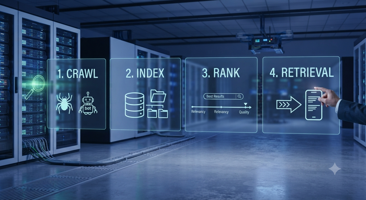
The data is in. Now the real question: someone types “atention is all yu need” — three typos — and you must find the right record among 8.6 million in a few milliseconds. Welcome to information retrieval (IR), the science behind every search box.
8. Index & Inverted Index
Why search is instantWithout an index, answering a query means reading all 8.6 million records front to back — a full scan that takes minutes (a real full pass over a multi-GB dataset can easily take over 2 minutes even on a fast machine). With an index, you jump straight to the answer. Take three tiny documents:
| Doc ID | Title |
|---|---|
| D1 | Attention Is All You Need |
| D2 | Neural Machine Translation |
| D3 | Attention in Neural Networks |
The forward direction is document → words. The inverted index flips (“inverts”) it to word → documents:
| Word | Appears in (the “posting list”) |
|---|---|
| attention | D1, D3 |
| neural | D2, D3 |
| translation | D2 |
| need | D1 |
Query “neural attention”? Look up both words, intersect the lists: {D2, D3} ∩ {D1, D3} = {D3}. Two dictionary lookups and one intersection — no matter whether you have 3 documents or 8.6 million.
In SQLite this whole machine is one line — the FTS5 module builds and maintains the inverted index for you:
<span class="k">CREATE VIRTUAL TABLE</span> records_fts <span class="k">USING</span> fts5(title, authors);
<span class="c">-- later: instant full-text search over millions of rows</span>
<span class="k">SELECT</span> * <span class="k">FROM</span> records_fts <span class="k">WHERE</span> records_fts <span class="k">MATCH</span> 'neural attention';9. BM25 — the Classic Ranking Formula
Scoring resultsMatching the word “the” with a record tells you almost nothing — millions of records contain it. Matching a rare surname like “Vaswani” tells you a lot — only a handful do. BM25 (Best Matching 25, invented in the 1990s and still the default baseline in every serious search system) turns that intuition into a score built from three ingredients:
| Ingredient | Question it asks | Effect on score |
|---|---|---|
| IDF (rarity) | How rare is this word across ALL records? | Rare word (“vaswani”) → big weight. Common word (“the”) → weight near 0. |
| TF (frequency) | How often does it appear in THIS record? | More is better — but with diminishing returns (10 mentions isn’t 10× better than 1). |
| Length normalization | Is this record unusually long? | Long records get slightly discounted, so they can’t win just by containing everything. |
Worked example — query: attention vaswani, against a 1-million-record collection:
| Word | Records containing it | Rarity weight (IDF, approx.) |
|---|---|---|
| the | 950,000 | ≈ 0.05 (worthless) |
| attention | 12,000 | ≈ 4.4 |
| vaswani | 45 | ≈ 10.0 (gold) |
A record containing both attention and vaswani scores ≈ 14.4 and rockets to rank 1; a record containing only the scores ≈ 0.05 and vanishes. That’s the whole trick.
10. Candidate Generation → Reranking (the Funnel)
Two-stage searchWhy two stages? Because your smartest matcher (a neural model, or an LLM comparing full records) might take 50 ms per record. Running it on 8.6 million records = 5 days per query. Running it on 100 candidates = half a second. The funnel is how every modern search engine, recommender, and matching system is built:
| Stage 1: Candidates | Stage 2: Reranking | |
|---|---|---|
| Input size | 8,600,000 | ~100 |
| Cost per record | microseconds (index lookup) | milliseconds (deep comparison) |
| Job | Don’t lose the right answer (high recall) | Put the right answer first (high precision) |
| Acceptable errors | 90 wrong candidates? Fine. | Wrong #1? Failure. |
Crucial insight: Stage 1 only has one job — never drop the correct record from the candidate list. If the truth isn’t among the 100, no amount of brilliant reranking can recover it. This connects directly to recall, coming up in section 13.
11. Edit Distance (Levenshtein) & Trigrams
Fuzzy / typo-tolerant matchingatention still matches attention. Edit distance counts keystrokes to fix a word; trigrams compare overlapping 3-letter chunks.Edit distance (Levenshtein distance)
The Levenshtein distance between two words is the minimum number of single-character edits — insert, delete, or substitute — needed to turn one into the other. Small distance = very similar.
| From → To | Edits needed | Distance |
|---|---|---|
atention → attention | insert one “t” | 1 |
jon → john | insert one “h” | 1 |
kitten → sitting | substitute k→s, e→i, insert g | 3 |
graph → graph | none | 0 |
Trigrams (character 3-grams)
A trigram is any run of 3 consecutive characters. Break both strings into trigram sets and measure how much they overlap — fast, and great for catching typos and partial titles. The word graph becomes:
"graph"  →  { <span class="k">gra</span> , <span class="k">rap</span> , <span class="k">aph</span> }
"graphs" →  { <span class="k">gra</span> , <span class="k">rap</span> , <span class="k">aph</span> , <span class="k">phs</span> }

shared trigrams: 3   ·   total distinct: 4
similarity = 3 / 4 = <span class="k">0.75</span> → strong match despite the extra letter| Edit distance | Trigrams | |
|---|---|---|
| Measures | exact keystrokes to fix | overlap of 3-char chunks |
| Best at | short strings, names | longer text, partial titles |
| Speed | slower (compares whole words) | fast (set overlap, index-friendly) |
12. Top-k Accuracy & MRR
Success metricsSay you run 4 test queries where you already know the correct answer. You record the position at which the correct answer appeared:
| Query | Correct answer landed at rank… | In Top-1? | In Top-5? | Reciprocal rank (1 ÷ rank) |
|---|---|---|---|---|
| Q1 | 1 | ✅ | ✅ | 1 / 1 = 1.00 |
| Q2 | 3 | ❌ | ✅ | 1 / 3 = 0.33 |
| Q3 | 2 | ❌ | ✅ | 1 / 2 = 0.50 |
| Q4 | 8 | ❌ | ❌ | 1 / 8 = 0.125 |
Top-1 accuracy = 1 of 4 = 25%. Top-5 accuracy = 3 of 4 = 75%. MRR (Mean Reciprocal Rank) = average of the last column = (1 + 0.33 + 0.50 + 0.125) ÷ 4 = 0.49.
Which to use? Top-1 matters when you show a single answer. Top-5 matters when the user sees a short list. MRR summarizes overall ranking quality in one number, which makes comparing two search methods easy.
13. Precision vs Recall
The eternal trade-offImagine a collection contains 10 records that are truly relevant to a query. Your system returns 8 records; 6 of them are actually relevant.
| Quantity | Value |
|---|---|
| Results you returned | 8 |
| …that were actually relevant (correct) | 6 |
| …that were wrong (false alarms) | 2 |
| Relevant records you missed entirely | 4 |
| Precision = 6 correct ÷ 8 returned | 75% |
| Recall = 6 found ÷ 10 that exist | 60% |
The trade-off. Return more results and you’ll catch more of the truly relevant ones (recall ↑) but also let in more junk (precision ↓). Return fewer, safer results and precision rises while recall falls. This is exactly why the two-stage funnel works: Stage 1 is tuned for high recall (don’t miss the answer), Stage 2 is tuned for high precision (put the right one first).
14. Baseline
The bar to beatBefore building anything sophisticated, you measure a plain method on the exact same test set. Then every new idea is judged by one question: did it beat the baseline?
| Method | Complexity | Top-5 accuracy | Verdict |
|---|---|---|---|
| Baseline (built-in fuzzy search) | none — it already exists | 62% | the bar 📏 |
| BM25 index | low | 71% | ✅ beats baseline |
| BM25 + trigram fuzzy | medium | 78% | ✅ better |
| Embeddings + reranking | high (slow, GPU) | 64% | ⚠️ barely beats baseline — not worth the cost |
Part 3 · Bonus — Six More Terms Every Data Project Uses
The two phases above are the core. But real pipelines lean on a handful of extra ideas constantly. Here are six worth knowing, each in one screen.
15. Checksum & Integrity
Did the file arrive intact?You run the same math on the official file and your downloaded copy. Identical fingerprints = identical bytes. One flipped bit produces a completely different fingerprint.
MD5 is fine for catching accidental corruption; SHA-256 is the stronger choice for security.Integrity is the bigger goal — data hasn’t been damaged or truncated — and a checksum is just one of several independent checks (is the archive readable? is the XML valid? do the counts reconcile?). No single check is enough; you layer them.
16. Transactions & Atomicity
All-or-nothing writesOne catalog record might need writes to 4 tables (the record, its authors, its fields, its links). If the power dies after write 2 of 4, you’d have a broken half-record. A transaction prevents that: nothing is saved until the whole group is confirmed.
<span class="k">BEGIN</span>;                               <span class="c">-- start the all-or-nothing block</span>
  <span class="k">INSERT INTO</span> records      VALUES (...);
  <span class="k">INSERT INTO</span> authors      VALUES (...);
  <span class="k">INSERT INTO</span> field_links  VALUES (...);
<span class="k">COMMIT</span>;                              <span class="c">-- ✅ all saved together</span>
<span class="c">-- if anything failed above → ROLLBACK undoes the whole block</span>
The classic analogy is a bank transfer: money must leave one account and arrive in the other, or neither. A checkpoint extends this idea to huge imports — you commit in groups (say, every 1,000 records) and record the last safely-saved position, so a crash never leaves the database and your progress-marker disagreeing.
17. Raw vs Normalized vs Derived Data
Keep the original untouched| Kind | Example value | Purpose |
|---|---|---|
| Raw / source | "An <i>Important</i> Result" | the untouchable truth from the source |
| Plain | "An Important Result" | markup stripped, still faithful |
| Normalized | "important result" | lowercased, for fast comparison |
| Derived | tokens, trigrams, embedding vector | computed features for search |
Why so careful? Normalization loses information. "J. Smith Jr." normalized to "j smith" is great for matching but has dropped the “Jr.” Store the normalized form alongside the original, never instead of it. (This is the data-level cousin of immutability from section 5.)
18. Provenance
Where did this value come from?When your system shows a user a title, provenance lets it also answer: Which source gave us this? Was it copied verbatim or cleaned? Can we show the original? That traceability is what makes a system trustworthy rather than a black box.
19. Federated vs Merged
Combining multiple sources| Merged | Federated | |
|---|---|---|
| Keeps originals? | ❌ overwrites into one | ✅ keeps each source |
| Conflicts | hidden — you can’t tell who said what | visible — “Source A says 2020, Source B says 2021” |
| Add a new source | risky re-merge | plug in a new adapter |
| Trace a mistake | hard | easy (see provenance) |
An adapter is the translator that converts one source’s format (XML, JSON, CSV…) into your common internal shape, so the rest of the system doesn’t care where a record originally came from. Federated systems link records that look like the same work rather than destructively fusing them — you can always build a merged “view” later, but you can’t un-merge once you’ve thrown originals away.
20. Embeddings, Rank Fusion, Calibration & Abstention
The modern matching toolkitEmbedding — turns text into a list of numbers (a vector) that captures meaning, so "heart attack" and "myocardial infarction" land close together even though they share no words. Word-matching (BM25) can’t do that; embeddings can. They complement lexical search rather than replacing it.
Rank fusion (RRF) — you often run several searchers (BM25, fuzzy, embeddings) that each produce a ranked list. Reciprocal-Rank Fusion combines them: a record ranked highly by several methods rises to the top. Consensus beats any single opinion.
Calibration — asks whether a confidence score is honest. If your system says “90% sure” on a batch of results, are about 90% of them actually right? A calibrated score you can trust; an uncalibrated “0.9” is just a number.
Abstention — the discipline of returning “no reliable match found” instead of forcing a wrong answer. For citations, medicine, or law, a confident wrong answer is far worse than an honest “I don’t know.”
Quick-Reference Glossary
Every term in one place — skim it before a discussion or an exam.
| Term | One-line definition |
|---|---|
| Streaming | Process a huge file one record at a time; memory stays flat. |
| Parsing | Turn raw text into validated, structured objects. |
| DTD / entity | XML’s grammar rulebook; é is a nickname for é. |
| Schema / ingestion | The database floor plan; moving data into it. |
| Immutability | Frozen objects that can’t be silently changed — protects source truth. |
| Reconciliation | Counts must match exactly: in = out + explained skips. |
| Census | Count your dataset by category and know the headline numbers cold. |
| Inverted index | Word → list of records containing it; makes search instant. |
| BM25 | Ranking formula where rare shared words count more than common ones. |
| Candidate → rerank | Cheap search narrows millions → ~100; expensive scoring picks the winner. |
| Edit distance | Keystrokes needed to turn one word into another (typo tolerance). |
| Trigram | Overlapping 3-character chunks; compare by how many they share. |
| Top-k accuracy | Was the correct answer in the top k results? (yes/no) |
| MRR | Mean reciprocal rank: on average, how high did the answer rank? |
| Precision | Of results returned, how many were right? (cleanliness) |
| Recall | Of all right answers, how many did you find? (completeness) |
| Baseline | The simple method every fancy method must beat. |
| Checksum | A file’s byte-fingerprint; match it to confirm an intact download. |
| Transaction / atomicity | A group of writes that all succeed or all get undone. |
| Raw / normalized / derived | Original vs tidied-for-matching vs computed values — kept separate. |
| Provenance | A value’s paper trail: source, field, and transformations. |
| Federated vs merged | Keep and link each source vs blend into one and lose originals. |
| Embedding | Text turned into numbers that capture meaning; search by concept. |
| Rank fusion (RRF) | Combine several ranked lists; consensus rises to the top. |
| Calibration | Whether a “90% sure” score is actually right ~90% of the time. |
| Abstention | Returning “no reliable match” instead of a confident wrong answer. |
Putting It All Together
Every search system you use runs the same two-act play. Act one gets data in safely: stream it, parse it, decode its grammar, pour it into a schema, freeze the originals, and reconcile the counts until every record is accounted for. Act two finds things fast: build an inverted index, rank with BM25, funnel millions of candidates down to one through reranking, tolerate typos with edit distance and trigrams, and measure yourself honestly with top-k, MRR, precision, recall — always against a baseline.
Learn these 26 terms and you can read the architecture of almost any search engine, database pipeline, or matching system — and build your own.