From 5 GB of XML to Instant Search
The eight steps of safely turning a giant public dataset into a searchable SQL database — explained for complete beginners, with one worked example the whole way through.
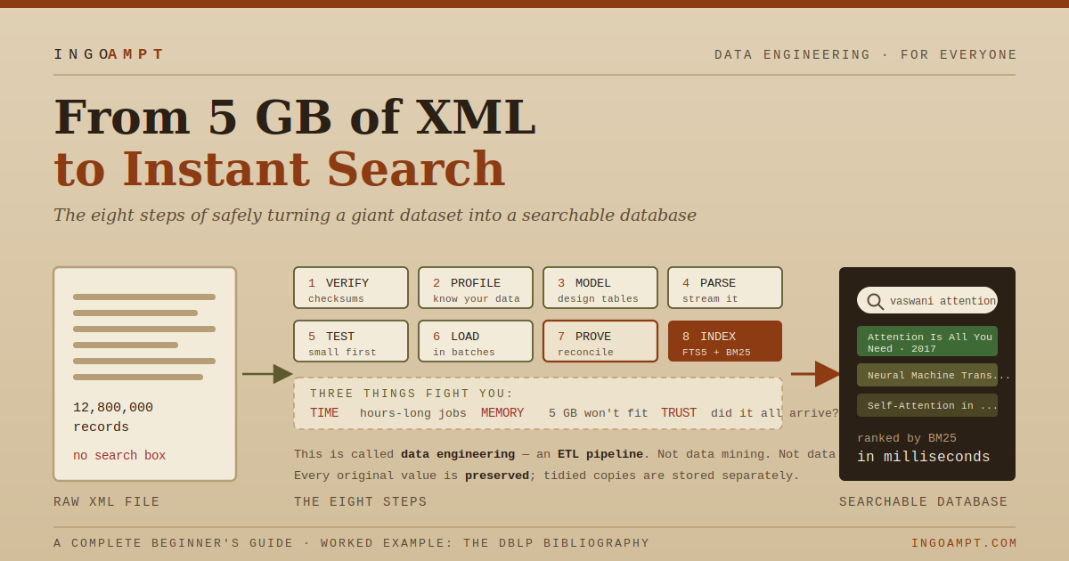
Imagine you download one file that contains almost every computer-science paper ever published: titles, authors, years, venues, DOIs. That file really exists. It is the DBLP computer-science bibliography, distributed as a single XML file that is roughly 1 GB compressed and about 5 GB when unpacked, holding on the order of 8.5 million publication records (plus millions of author and link entities — which is why people often say “over 12 million records”).
You can open it in a text editor and see the data. But you cannot ask it a question. There is no search box. Type “find every paper by this author from 2019” and the file just sits there, silent.
This article is the recipe for fixing that — turning an enormous, unsearchable file into a small, fast, searchable database, safely, meaning without corrupting or silently altering a single original value. We will use one running example all the way through: let us imagine we want to convert the DBLP XML dump into SQLite safely. Every step, though, is a reusable recipe you can apply to your own data: a government open-data dump, a Wikipedia export, a museum catalog, your company’s legacy records.
You are not going to “clean” the data by editing it in place. You are going to preserve every original value exactly as it came, and store any tidied-up or search-friendly versions separately, clearly labelled as derived. That single discipline is what separates a trustworthy dataset from a mystery file.
STEP 1Get the source and prove it is intact
Industry name: source verification · integrity checking · checksum validation
What it is
Before you process a single byte, you download the file and prove it arrived complete and unmodified. The tool is a checksum (also called a hash): a short fingerprint such as an MD5 or SHA-256 string that changes completely if even one bit of the file changes. You also record provenance: where the file came from, when you downloaded it, and which exact version it is.
Why it matters
Downloads get truncated. Disks flip bits. Files get swapped. If your source is silently broken, everything you build on top is built on sand — and you will not discover it for weeks. A checksum gives you near-mathematical certainty that your copy matches the publisher’s copy. MD5 is fine for catching accidental corruption; SHA-256 is the safer choice when tampering matters.
The DBLP example
DBLP publishes three files side by side: dblp.xml.gz (the data), dblp.xml.gz.md5 (its checksum) and dblp.dtd (the grammar file the parser needs). The safe routine:
- Download all three from the official directory.
- Recompute the MD5 of your
.gzand compare it with the published one. - Test the archive itself with
gzip -tbefore unpacking. - Write down the provenance. DBLP publishes monthly snapshots with their own DOIs, and recommends citing the snapshot rather than the ever-changing daily file — so your work stays reproducible. Note also the licence: DBLP’s metadata is released under CC0 (public domain), so reuse is free.
STEP 2Look before you leap
Industry name: data profiling · data auditing
What it is
Data profiling means examining the raw data to learn its real shape before you design anything. How many records? Which record types exist? Which fields appear, and how often? Any duplicates or missing keys? And — crucially — you open a handful of real records and read them with your own eyes.
Why it matters
Migration guides call a thorough data audit “one of the most critical yet often underestimated best practices… before moving a single byte.” Skip it and you are migrating data you do not understand; you will discover its surprises only after the load, when fixing them is expensive. Profiling is how you replace assumptions with numbers.
The DBLP example
A profiling pass over DBLP reveals facts that directly shape the design: the collection is dominated by conference papers (inproceedings, roughly 3.9 million, about 46%) and journal articles (about 3.4 million, roughly 40%), with a large informal/preprint category (around 921,000) and smaller counts of books, theses and data records. It also reveals traps: www records look like publications but are actually author home pages; a single paper carries many <author> elements in a meaningful order; and DOIs hide inside <ee> link fields rather than a tidy doi column.
STEP 3Design the destination
Industry name: schema design · data modelling
What it is
Schema design is deciding the tables, columns, keys and relationships in your target database, and writing down the mapping from the source’s shape to that structure. XML is a tree; SQL is tables; somebody has to translate, deliberately.
Why it matters
Do it well and queries are fast and honest. Do it carelessly and you silently lose information — most famously ordering. Three professional rules apply: preserve ordered relationships, keep original values separate from derived ones, and store provenance inside the data so every row can be traced to the exact snapshot it came from.
The DBLP example
- A
publicationstable: one row per record, keyed by the DBLP key, withtype,title,year,venue,doi. - An
authorstable plus apublication_authorsjoin table — with an explicitauthor_positioncolumn, because in science first and last author mean different things. Tables have no built-in row order, so if order matters you must store it as data. - Provenance columns: snapshot DOI, source checksum, import date.
- Original vs derived: keep the exact original title; if you later build a lowercased, punctuation-stripped version for searching, put it in a separate column such as
title_normalizedand never overwrite the original.
STEP 4Build the reader
Industry name: parsing · extraction (the E of ETL)
What it is
Now you write the code that reads the XML and produces rows. For huge files the technique is streaming parsing (SAX, or iterparse in Python): process one record at a time, then throw it away — instead of loading the whole 5 GB tree into memory.
Why it matters
A DOM parser loads the entire document into RAM, typically needing several times the file size. On a normal laptop that is an instant crash. Streaming keeps memory bounded and flat: one record at a time, forever. You also want each write wrapped in a transaction so a crash can never leave half a record behind.
The DBLP example
Use iterparse with one crucial detail: after handling each record element, call elem.clear() to free it — the classic beginner mistake is letting parsed elements pile up until memory dies. DBLP adds two specific gotchas: the dblp.dtd is a “private” resource you must download and keep next to the XML (it defines the character entities such as accented letters), and because the file contains an enormous number of entities, parsers may need their entity-expansion security limit raised. Each parsed record becomes a small immutable object (key, title, year, ordered authors) handed to the loader.
STEP 5Test small first
Industry name: staged validation · sample loads · dry run
What it is
Before the multi-hour full load, run the entire pipeline on small samples — say 1,000 records, then 100,000 — and validate the output each time.
Why it matters
Validation is not something you save for the end; it starts before the migration does. Catching a mapping bug on 1,000 records costs seconds. Catching the same bug after a full load costs the entire run — and your afternoon. Small runs also give you the two numbers you need to plan the big one: records per second and bytes per record.
The DBLP example
Load the first 1,000 records into a throwaway database and check: does the row count match, minus any record types you deliberately skip? Do a few known papers have their authors in the right order? Did the DOI land in the right column when <ee> contained one? Then scale to 100,000, watch memory and speed, and multiply out: if 100,000 records take one minute and 220 MB, then 8.5 million will take roughly an hour and a few gigabytes. Only then commit to the real run.
STEP 6Run the full load
Industry name: loading · ingestion · bulk load (the L of ETL)
What it is
Parsing every record and inserting it into the database, for real — the hours-long unattended run.
Why it matters
At millions of records, how you insert dominates everything. Three ideas make the difference between a job that finishes and one that ruins your day:
- Batched transactions. A transaction is a group of writes that all succeed or all un-happen. Committing one record at a time is agonisingly slow (the database must force each one to disk); committing everything in one giant transaction means a crash at 90% loses everything. Committing every 1,000–10,000 records captures nearly all the speed while capping what a crash can cost.
- Checkpoints. After each committed batch, durably record a bookmark: “complete through record 6,000,000.” On restart, resume there instead of at zero.
- Do not build search indexes yet. Indexes must be updated on every single insert. Load first, index at the end (that is Step 8).
STEP 7Prove it is correct
Industry name: reconciliation · data validation · data quality checks
This is where amateurs stop and professionals begin. The importer printing “Done!” tells you the program finished. It does not tell you the data is correct. Step 7 is how you turn belief into evidence — and it is genuinely the easiest step of all, because you are only counting and comparing.
7.1 What reconciliation means
Data reconciliation is the formal process of verifying a migration by comparing the source against the target. It is normally the final step of any migration test. Six checks, from cheapest to deepest:
| Check | Question it answers | How |
|---|---|---|
| 1. Total count | Did every record arrive? | Records read from the source vs. rows written to the database |
| 2. Per-type counts | Did one kind of record go missing? | Compare article / inproceedings / book / thesis counts separately |
| 3. Key uniqueness | Any duplicates or collisions? | Group by key, expect zero groups larger than one |
| 4. Referential integrity | Any orphan links? | PRAGMA foreign_key_check — every author link must point at a real record |
| 5. Physical integrity | Is the file itself sound? | PRAGMA integrity_check (or the faster quick_check) |
| 6. Sampling | Are the contents right, not just the count? | Pull random records, compare field by field with the raw source |
7.2 Why two independent counts are strong evidence
Checks 1 and 2 rest on a 600-year-old idea: double-entry bookkeeping. Accountants record every transaction twice, from two directions, and the totals must agree; a mismatch is a guaranteed sign of an error. Here, one count comes from scanning the source file, the other from querying the database — two different tools, two different code paths, two different moments in time. For both to be wrong in exactly the same way is essentially impossible. That is why agreement is proof rather than hope.
7.3 The manifest: your database’s birth certificate
When reconciliation passes, write a manifest and store it with the database. It records:
- source filename, snapshot version/DOI and its checksum;
- the code version that built it (for example a git commit hash);
- the settings used (batch size, profile, options);
- start and finish time, runtime, throughput;
- final record counts and database size.
This is what makes your result reproducible: somebody else — or future you — can rebuild the identical database and get identical numbers. It also satisfies the “Reusable” pillar of the widely-adopted FAIR data principles (Findable, Accessible, Interoperable, Reusable), which asks for clear provenance, quality and licensing information.
“The importer finished” is not the definition of done. Done means: counts reconcile (total and per type), keys are unique, foreign-key and file-integrity checks pass, spot-checks match the source, and the manifest is written. Anything less is a database you hope is right.
STEP 8Make it searchable
Industry name: indexing · full-text search · information retrieval
You now have a correct, verified database. It is still not fast to search. This step is where a pile of data becomes a search engine — and it is the part most tutorials never reach.
8.1 Why a loaded database is still slow
Run SELECT * FROM publications WHERE title LIKE '%neural%' and the database must perform a full table scan: read every one of the millions of rows, examine each title, and test for the substring. There is no shortcut, because a search pattern beginning with % cannot use an index. It is slow, it cannot rank results, and it cannot match word variants.
8.2 B-tree indexes: jump instead of crawl
An index is the back-of-the-book index for your table: a pre-sorted structure that lets the engine jump straight to matching rows. SQL indexes are B-trees — balanced trees that discard a large chunk of candidates at every hop, so finding one value among a million rows takes on the order of twenty comparisons rather than a million.
They are perfect for exact and range lookups: WHERE year = 2019, WHERE doi = '10.1145/...', WHERE year BETWEEN 2010 AND 2015. The costs are real but manageable: writes get slower (every insert must update every index — which is exactly why Step 6 said load first, index later) and each index takes disk space. So you index only the columns you actually search or join on.
8.3 Try the identifier first — the fastest path of all
Before any text search, ask: do I have an identifier? A DOI, arXiv ID, ISBN or the source’s own key uniquely identifies a record. Looking one up against a B-tree index is instant and unambiguous — no guessing, no ranking, no false matches. Production matching systems always try identifiers first and fall back to text search only when there is no identifier to use.
8.4 Full-text search with SQLite FTS5
For real text search (“papers about attention transformers”), SQLite ships a dedicated engine: FTS5, a virtual-table module that has been part of SQLite since version 3.9.0 (2015). Instead of scanning, it builds an inverted index — a map from each word to the list of rows containing it — and ranks results with BM25 out of the box.
Creating the search table is one statement:
CREATE VIRTUAL TABLE pub_fts USING fts5(title, venue);Do not store your text twice. By default FTS5 keeps its own copy of the text, which for millions of rows doubles storage. The fix is an external content table: FTS5 stores only the index and reads the actual values from your existing table.
CREATE VIRTUAL TABLE pub_fts USING fts5(
    title, venue,
    content='publications',
    content_rowid='id'
);
Searching uses the MATCH operator, and you can mix it freely with ordinary SQL conditions:
SELECT title FROM pub_fts
WHERE pub_fts MATCH 'neural attention'
ORDER BY rank
LIMIT 10;
The query language supports phrases ("deep learning"), boolean AND/OR/NOT, prefix search (transform* matches transformer, transformation), column filters (title:neural) and proximity search.
| Tokenizer | What it does | Use it when |
|---|---|---|
unicode61 (default) | Sensible Unicode word splitting, case-insensitive | Almost always — the safe default |
ascii | Treats only ASCII characters as special | Plain English-only data |
porter | Adds stemming: running / runs / run fold together | You want word variants to match |
trigram | Indexes 3-character sequences, enabling substring and typo-tolerant matching | You need to match fragments inside words |
8.5 Populating and maintaining the index
Build the index after the bulk load. With an external-content table you fill it with one special command, then compact it:
INSERT INTO pub_fts(pub_fts) VALUES('rebuild');
INSERT INTO pub_fts(pub_fts) VALUES('optimize');
rebuild deletes the whole index and regenerates it from the content table (it is also the repair tool if the two ever drift apart). optimize merges the index into a single compact structure — the smallest on disk and the fastest to query. Both take a while on millions of rows; both are one-time costs.
8.6 BM25 ranking, explained simply
Finding matches is only half the job; ordering them is the other half. BM25 is the classic ranking function used by full-text search engines — the same family used by Elasticsearch and Lucene — and FTS5 has it built in. It scores each result using three intuitions:
8.7 Normalised text for search — kept separate from the originals
To make search robust you index a normalised copy of the text: lowercased, punctuation and markup stripped, disambiguation suffixes removed (bibliographies often append numbers to distinguish authors with identical names — useful for identity, noise for search). Following the Step 3 rule, these normalised strings live in separate columns; the authoritative original is never overwritten. You search the normalised copy and display the original.
8.8 What comes after BM25
| Technique | What it adds |
|---|---|
| Fuzzy / trigram matching | Tolerates typos and partial words (“atention” still finds “attention”) |
| Embeddings / semantic search | Matches meaning, so “car” can find “automobile” with no shared words |
| Hybrid retrieval + rank fusion (RRF) | Runs keyword and semantic search together and merges the two ranked lists |
| Reranking | Passes the top 50–100 candidates to a slower, smarter model for a final precise order |
| Calibrated confidence | Turns raw scores into an honest “92% sure” the user can trust |
| Evaluation metrics | Top-1 / Top-5 accuracy, MRR and Recall@k — how you prove one method beats another |
What is all this actually called?
Terminology — and three things this is NOT
Beginners get lost because the field has many overlapping words, often used loosely. Here is the precise map.
The umbrella term is data engineering: building the systems that move and prepare data for use. The specific pattern in this article is an ETL pipeline — Extract (parse the XML), Transform (map it to tables, derive normalised copies), Load (insert into the database). Its cousin ELT loads raw data first and transforms it inside a big warehouse afterwards, which is common in cloud data platforms. The whole automated flow is a data pipeline; the one-time mass move is a data migration or bulk load.
| Our step | What it is called in industry |
|---|---|
| 1. Get and verify the source | source verification, integrity checking, checksum validation |
| 2. Look before you leap | data profiling, data auditing |
| 3. Design the destination | schema design, data modelling |
| 4. Build the reader | parsing, extraction (streaming / SAX / iterparse) |
| 5. Test small first | staged validation, sample loads, dry run |
| 6. Run the full load | loading, ingestion, bulk load |
| 7. Prove it is correct | reconciliation, data validation, data quality checks |
| 8a. Speed up lookups | indexing (B-tree) |
| 8b. Search the text | full-text search, information retrieval |
Three distinctions worth memorising
| Term | What it means | Is that what we did? |
|---|---|---|
| Data engineering / ETL | Building the pipeline that moves and prepares data | YES — this is the correct name |
| Data mining | Discovering unknown patterns and relationships in data that is already stored | NO — that comes after, on top of the database |
| Data cleaning / cleansing | Correcting errors: removing duplicates, fixing values, filling gaps — it changes the data | NO — we deliberately preserve every original value |
| Data wrangling / munging | The broad reshaping of raw data into a usable form (cleaning is a part of it) | Partly — our transform step is a mild form of it |
| Data curation | Organising, describing, preserving and adding value to data over its lifetime | YES — our provenance and manifest discipline is exactly this |
If you correct a value inside your copy of a published dataset, your database no longer matches the source, and nobody — including you — can tell later which values were original and which you altered. Provenance dies, reproducibility dies. The professional alternative is what this article does throughout: preserve the original, add a derived column, and document the derivation. Cleaning is legitimate work — it just belongs in a clearly-labelled derived layer, never in place.
The reusable checklist for your own data
Lift this for any dataset: open government data, a Wikipedia export, a product catalogue, legacy records
Before you load
- Acquire and verify. Download the data and its checksum; recompute and compare; test the archive; record source URL, version/DOI, date, size, checksum — and check the licence.
- Profile before designing. Count records and types; measure field coverage; look for duplicates and missing keys; read real samples with your own eyes.
- Model the target. Design tables, keys, relationships. Store ordering as data. Keep original and derived values separate. Add provenance columns.
While you load
- Stream, never slurp. Parse incrementally and release each record after use.
- Rehearse on samples. 1,000 then 100,000 records; validate counts, mapping, ordering; measure speed and size to predict the full run.
- Load in batches with checkpoints so an interruption resumes instead of restarting.
- Do not build search indexes yet.
After you load
- Reconcile. Source vs target counts, total and per type; key uniqueness; foreign-key check; integrity check; sample spot-checks.
- Write the manifest: source + checksum, code version, settings, runtime, counts, size.
- Then build search. B-tree indexes on what you query and join; identifier lookup first; FTS5 with an external content table;
rebuildthenoptimize; order by rank.
Always
- Right-size the effort to the stakes. A throwaway CSV needs almost none of this. A dataset that a publication, a product or a decision depends on needs most of it. Knowing which situation you are in is the real skill.
What comes next
Once a searchable database exists, the natural continuations are short to describe and long to perfect: evaluate search quality against a small benchmark of known question-answer pairs (Top-1, Top-5, MRR); add better matchers (fuzzy, semantic, hybrid, reranking); put an interface on top — a search box, an API; and decide how to stay fresh when the source publishes a new release: a full rebuild from the new snapshot (simplest and safest while it is cheap) or incremental updates that apply only the changes (necessary once rebuilding becomes too slow — and remember that increments must handle deletions, not only additions).
Closing thought
“Just load the file into a database” hides an entire discipline. What actually happens is a small logistics campaign against three adversaries — time, memory and trust — fought with checksums, streaming parsers, batched transactions, checkpoints, reconciliation and indexes. None of the eight steps is difficult on its own. What separates an experienced engineer from a frustrated beginner is doing them in the right order, proving each one before moving on, and knowing which of them a given job actually needs.
Do that, and a silent 5 GB file becomes something genuinely valuable: a database that answers in milliseconds, tells you where every value came from, and can be rebuilt by anyone, exactly, from the source.
Further reading
SQLite documentation — the FTS5 extension (virtual tables, bm25(), rank, tokenizers, external-content tables, rebuild and optimize), query planning and indexing, and the PRAGMA reference for integrity_check and foreign_key_check (sqlite.org) · DBLP’s own FAQ and blog on parsing dblp.xml, the DTD, monthly DOI snapshots and the CC0 licence (dblp.org, blog.dblp.org) · Okapi BM25 and information-retrieval evaluation metrics — Introduction to Information Retrieval by Manning, Raghavan and Schütze · the FAIR Guiding Principles for scientific data management (Wilkinson et al., Scientific Data, 2016) · data-migration best-practice guides on profiling and reconciliation as standard pre- and post-migration steps · Cormack, Clarke and Büttcher, “Reciprocal Rank Fusion” (SIGIR 2009) for hybrid-search fusion.
A note on the numbers: dataset sizes and record counts grow every month, so treat all figures here as a snapshot rather than a constant — which is precisely why Step 1 insists you record the exact version you used. Figures in this article are original illustrations.