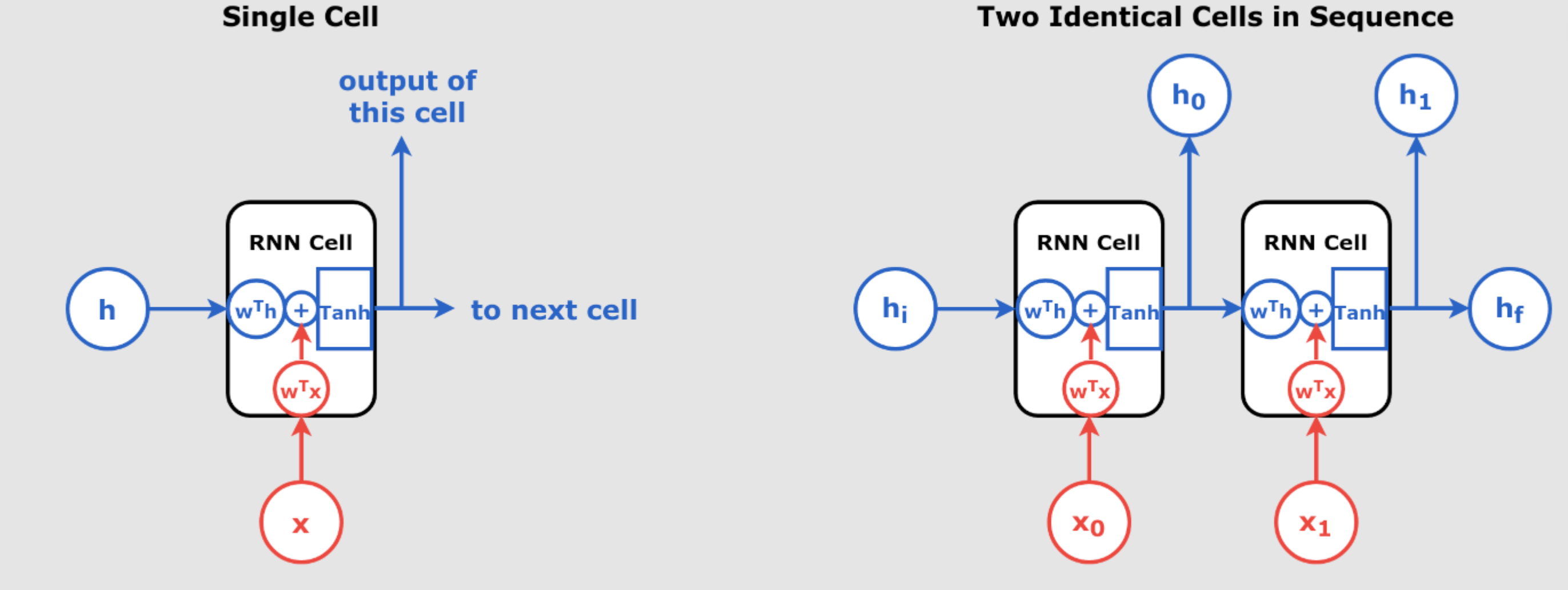
A Deep Dive into Recurrent Neural Networks, Layer Normalization, and LSTMs

So far we have explained in pervious days articles a lot about RNN. We have explained, Recurrent Neural Networks (RNNs) are a cornerstone in handling sequential data, ranging from time series analysis to natural language processing. However, training RNNs comes with challenges, particularly when dealing with long sequences and issues like unstable gradients. This post will cover how Layer Normalization (LN) addresses these challenges and how Long Short-Term Memory (LSTM) networks provide a more robust solution to memory retention in sequence models.

The Challenges of RNNs: Long Sequences and Unstable Gradients

When training an RNN over long sequences, the network can experience the unstable gradient problem—where gradients either explode or vanish during backpropagation. This makes training unstable and inefficient. Additionally, RNNs may start to “forget” earlier inputs as they move forward through the sequence, leading to poor retention of important data points, a phenomenon referred to as the short-term memory problem.

Addressing Unstable Gradients:

• Gradient Clipping: Limits the maximum value of gradients, ensuring they don’t grow excessively large.
• Smaller Learning Rates: Using a smaller learning rate helps prevent gradients from overshooting during updates.
• Activation Functions: Saturating activation functions like the hyperbolic tangent (tanh) help control gradients better than ReLU in RNNs.
• Layer Normalization: As we’ll explore further, layer normalization is particularly well-suited to address this issue in RNNs.

Why Batch Normalization Doesn’t Work Well with RNNs

As we have explain in our pervious articles , Batch Normalization (BN) is a technique designed to improve the training of deep neural networks by normalizing the inputs of each layer so that they have a mean of zero and a variance of one. This process addresses the issue of internal covariate shift, where the distribution of each layer’s inputs changes during training, potentially slowing down the training process. By stabilizing these input distributions, BN allows for higher learning rates and accelerates convergence.

However, BN does not work as effectively in RNNs for several reasons:

• Temporal Dependence: In RNNs, hidden states evolve over time, making it difficult to normalize across mini-batches at each time step.
• Small Batches in Sequential Data: BN requires large batch sizes to compute meaningful statistics, which is often impractical for RNNs that operate on smaller batch sizes or variable-length sequences.
• Sequence Variation: Since BN operates across mini-batches, it struggles to accommodate variable sequence lengths common in sequential tasks like text processing.

In contrast, Layer Normalization (LN) normalizes across features within each time step, allowing it to handle sequences efficiently.

Layer Normalization: The Solution for RNNs

Layer Normalization was introduced to solve some of the limitations of BN in RNNs. It operates by normalizing across the features within a layer, rather than across the mini-batch. This approach is particularly useful in RNNs because it:

• Layer Normalization (LN): Introduced by Ba et al., LN normalizes the inputs across the features within a single data sample rather than across the batch. This approach makes LN more suitable for RNNs, as it maintains the sequential dependencies and is effective even with small batch sizes.

  arXiv

• Assorted-Time Normalization (ATN): Proposed by Pospisil et al., ATN preserves information from multiple consecutive time steps and normalizes using them. This setup introduces longer time dependencies into the normalization process without adding new trainable parameters, enhancing the performance of RNNs on various tasks.

  arXiv

• Batch Layer Normalization (BLN): Ziaee and Çano introduced BLN as a combined version of batch and layer normalization. BLN adaptively weights mini-batch and feature normalization based on the inverse size of mini-batches, making it effective for both Convolutional and Recurrent Neural Networks.

  arXiv

Code Example for Layer Normalization :

class LNSimpleRNNCell(tf.keras.layers.Layer):
    def __init__(self, units, activation="tanh", **kwargs):
        super().__init__(**kwargs)
        self.state_size = units
        self.output_size = units
        self.simple_rnn_cell = tf.keras.layers.SimpleRNNCell(units, activation=None)
        self.layer_norm = tf.keras.layers.LayerNormalization()
        self.activation = tf.keras.activations.get(activation)

    def call(self, inputs, states):
        outputs, new_states = self.simple_rnn_cell(inputs, states)
        norm_outputs = self.activation(self.layer_norm(outputs))
        return norm_outputs, [norm_outputs]
  

How to Use It in a Model:

custom_ln_model = tf.keras.Sequential([
    tf.keras.layers.RNN(LNSimpleRNNCell(32), return_sequences=True, input_shape=[None, 5]),
    tf.keras.layers.Dense(14)
])

  

Explanation:

1. Initialization (__init__ method):

   • units: Specifies the number of units in the RNN cell.
   • activation: The activation function to apply after normalization.
   • simple_rnn_cell: An instance of SimpleRNNCell without an activation function.
   • layer_norm: An instance of LayerNormalization to normalize the outputs.
   • activation: Retrieves the activation function specified (default is “tanh”).

2. Forward Pass (call method):

   • inputs: The input tensor at the current time step.
   • states: The state tensor(s) from the previous time step.
   • The simple_rnn_cell processes the inputs and previous states to produce outputs and new_states.
   • outputs are then normalized using layer_norm.
   • The specified activation function is applied to the normalized outputs.
   • The method returns the activated, normalized outputs and the new state wrapped in a list.

custom_ln_model  in the code is a model integrates the custom LNSimpleRNNCell into a sequential model, followed by a dense layer with 14 units.

• Where Is Layer Normalization Applied?

  
  • Inside the call method:
     

    norm_outputs = self.activation(self.layer_norm(outputs))<br />
    • The outputs of the RNN cell (outputs) are normalized using self.layer_norm.
    • After normalization, the activation function (e.g., tanh) is applied to the normalized outputs.

• Why Layer Normalization Works Well Here?

  • Layer Normalization (LN) normalizes the inputs across features within a single data sample, maintaining sequential dependencies inherent in RNNs.
  • Unlike Batch Normalization, which computes statistics across batches, LN is effective for small batch sizes and sequences of varying lengths.

• Layer Normalization vs. Batch Normalization:

  • Layer Normalization (LN):

    • Normalizes the inputs across the features within a single data sample.
    • Particularly effective for RNNs as it maintains sequential dependencies and performs consistently regardless of batch size.
    • Applied independently at each time step, making it suitable for sequence modeling tasks.

  • Batch Normalization (BN):

    • Normalizes the inputs across the batch dimension for each feature.
    • Relies on batch statistics, which can be less effective for RNNs due to varying sequence lengths and dependencies.
    • More suited for feedforward neural networks and convolutional networks.

---

Lets Explain Deeper the Math Behind Layer Normalization vs Batch Normalization:

Layer Normalization (LN)

• Normalization Scope: LN normalizes across all the features (dimensions) of a single sample (or layer).
• Key Idea: Treats the entire feature vector of a sample as a unit and calculates the mean and standard deviation for the features within that sample.
• Analogy: Think of LN as looking at a single row of data (sample) and balancing all its feature values.

Example:

For a batch of samples:

    [
        [1, 2, 6],
        [4, 5, 8]
    ]
    

• LN computes the mean and standard deviation for each row independently:
• For Row 1: [1, 2, 6] → Mean = 3, Variance = 4.67 → Normalized: [-1.0, -0.5, 1.5].
• For Row 2: [4, 5, 8] → Mean = 5.67, Variance = 2.89 → Normalized: [-1.0, -0.39, 1.39].

Batch Normalization (BN)

• Normalization Scope: BN normalizes each feature independently, but across all samples in a batch.
• Key Idea: Treats each feature (column) as a unit and calculates the mean and standard deviation across the batch.
• Analogy: Think of BN as balancing each column of data (feature) across multiple rows (samples).

Example:

For the same batch of samples:

    [
        [1, 2, 6],
        [4, 5, 8]
    ]
    

• BN computes the mean and standard deviation for each column:
• Column 1: [1, 4] → Mean = 2.5, Variance = 2.25 → Normalized: [-1.0, 1.0].
• Column 2: [2, 5] → Mean = 3.5, Variance = 2.25 → Normalized: [-1.0, 1.0].
• Column 3: [6, 8] → Mean = 7, Variance = 1 → Normalized: [-1.0, 1.0].

Comparison Summary:

Aspect	Layer Normalization (LN)	Batch Normalization (BN)
Scope	Normalizes across features of a single sample.	Normalizes across samples for each feature.
Dependence on Batch	Independent of batch size.	Dependent on batch size.
Best For	Sequential models (RNNs, Transformers).	Feedforward/CNN models.
Key Operation	Considers a row (entire layer or sample).	Considers a column (feature across batch).

Visualization (Simplified Concept):

Layer Normalization (LN): Balances each row independently:

    Row 1: [1, 2, 6] → Normalize → [-1.0, -0.5, 1.5]
    Row 2: [4, 5, 8] → Normalize → [-1.0, -0.39, 1.39]
    

Batch Normalization (BN): Balances each column independently:

    Feature 1: [1, 4] → Normalize → [-1.0, 1.0]
    Feature 2: [2, 5] → Normalize → [-1.0, 1.0]
    Feature 3: [6, 8] → Normalize → [-1.0, 1.0]
    

As you can see in the provided example,

LN works on the entire feature vector (row) within a sample.

BN does not operate row by row. Instead, it normalizes each feature (column) across the batch.

All in all, LN is great for sequential models (like RNNs), while BN is typically better for convolutional or dense architectures.

Final Key Note to understand RNN better and why LN is better for RNN:

RNNs are fundamentally affected by rows rather than columns, and that is why Layer Normalization (LN), which normalizes rows, is better suited for RNNs than Batch Normalization (BN), which normalizes columns:

RNNs process data sequentially, focusing on one time step at a time, where each time step corresponds to a single row of features. This fundamental row-wise operation makes Layer Normalization (LN) more compatible with RNNs than Batch Normalization (BN). Here’s why:

---

1. RNNs Process Rows, Not Columns

• At each time step, the RNN processes one row of features representing the input at that moment.
• The RNN computes the hidden state for that time step using the current row and the hidden state from the previous time step.

This means that each row is treated as a distinct unit, and its features directly influence the hidden state. Consequently, ensuring that the features within each row are well-normalized is critical for stable and effective training.

---

2. LN Normalizes Rows

• Layer Normalization (LN) operates at the row level:
  • It computes the mean and variance across the features (columns) within a single row.
  • The normalization ensures that the input features at each time step are centered and scaled consistently.

This aligns perfectly with RNNs because:

• Each row (time step) is processed independently.
• LN ensures that the features of the current row do not depend on other rows, maintaining consistency.

---

3. BN Normalizes Columns

• Batch Normalization (BN) operates at the column level:
  • It computes the mean and variance of each feature (column) across all rows in the batch.
• This batch-wide dependency introduces two key issues for RNNs:
  1. Temporal Instability: The batch statistics can change significantly between time steps, disrupting the temporal dependencies that RNNs rely on.
  2. Dependency on Batch Size: RNNs often work with small batch sizes (or even single samples) due to memory constraints, making BN’s batch-wide statistics unreliable or inconsistent.

---

4. Temporal Dependencies in RNNs

• RNNs rely heavily on the stability of inputs across time steps to learn meaningful sequential patterns.
• LN ensures stable normalization for each time step because it normalizes independently for each row.
• BN, by contrast, introduces variability due to its reliance on batch-wide statistics, which may differ from one time step to another.

So I hope you could understand deeply why LN is better for RNN. We have fully explained that  RNNs process data row by row (time step by time step), making them fundamentally affected by rows rather than columns. LN’s row-based normalization aligns naturally with this structure, ensuring consistency and stability across time steps. In contrast, BN’s column-based normalization disrupts this temporal consistency, making LN the better choice for RNNs.

 

 

 

The Short-Term Memory Problem and LSTMs

Even with Layer Normalization (LN), standard RNNs often fail to retain important information over long sequences, which brings us to Long Short-Term Memory (LSTM) networks. LSTMs are specifically designed to address the short-term memory problem by maintaining two key states:

• Short-Term State (hₜ): Captures the most recent information at the current time step.
• Long-Term State (cₜ): Stores information over longer sequences, allowing the network to retain useful context for more extended periods.

Let’s simplify the explanation! LSTMs are like improved versions of RNNs. Both process data one row at a time, but LSTMs add a “memory system” that helps them remember important information from earlier rows while deciding what to forget or update at each step.

RNNs: Row-by-Row Basics

• RNNs handle sequential data (like sentences or time series) one row (or time step) at a time.
• At each time step:
  • RNNs take the current row (e.g., words in a sentence or data at a time step).
  • Combine it with what they remembered from the previous row (the “hidden state”).
  • Use this to calculate a new hidden state for the current row.
• Problem: RNNs can’t decide what to forget or remember, and over long sequences, they often forget earlier rows (this is called the vanishing gradient problem).

---

LSTMs Improve RNNs

LSTMs work like RNNs but add extra features to fix these problems:

• Memory Cell (A Notebook): Think of this as a notebook that keeps track of important information across rows (time steps).
• Gates (Decision Makers): LSTMs use gates to decide:
  1. What to forget from the memory.
  2. What new information to add to the memory.
  3. What to output for the current row.

These gates let LSTMs dynamically adjust how they process each row based on the current input and past information.

How LSTMs Process Rows (Step-by-Step)

At each row $t$:

1. Forget Gate:

   • Looks at the current row ($x_t$) and the hidden state from the previous row ($h_{t-1}$).
   • Decides how much of the previous memory to forget.

2. Input Gate:

   • Decides what new information from the current row ($x_t$) to add to the memory.

3. Update Memory:

   • Combines the forgotten information with the new information to update the memory.

4. Output Gate:

   • Decides what part of the updated memory to output as the hidden state for this row ($h_t$).

Why LSTMs Are Related to Row-by-Row Processing

• LSTMs, like RNNs, process one row at a time.
• The difference is:
  • RNNs just pass information forward without control, often losing important details.
  • LSTMs use the memory cell and gates to control the flow of information row by row.

Example to Clarify

Imagine you’re reading a story:

• RNNs: You read each line, but you don’t take notes. By the time you get to the last line, you forget what happened earlier.
• LSTMs: You read each line and take notes (memory cell). You decide:
  • What parts of the story to forget (e.g., unimportant details).
  • What new information to write down.
  • What to focus on for the next part of the story.

 

Key Takeaway

LSTMs are built on the row-by-row structure of RNNs but add a memory system and decision-making gates. This allows them to remember important information over long sequences and avoid forgetting or losing details like RNNs often do.

 

LSTM Structure: LSTMs introduce three gates—forget, input, and output—that control the flow of information, deciding which information to retain, which to discard, and what to output at each step.

LSTM Code Example:

model = tf.keras.Sequential([
    tf.keras.layers.LSTM(32, return_sequences=True, input_shape=[None, 5]),
    tf.keras.layers.Dense(14)
])

  

LSTMs use these gates to manage memory and retain long-term dependencies in the data, solving one of the most critical challenges in sequence modeling.

How Layer Normalization and LSTMs Improve RNNs

By combining Layer Normalization and LSTMs, we can build models that effectively handle long sequences and mitigate unstable gradients:

• Layer Normalization: Stabilizes the training process and ensures smooth gradient flow, preventing exploding or vanishing gradients.
• LSTMs: Allow the network to maintain long-term memory, enabling it to better understand long-range dependencies in the sequence data.

Both techniques work in harmony to tackle the primary weaknesses of traditional RNNs, making them essential tools for anyone working with sequential data like time series, language models, or any application requiring memory retention over time.

Detailed Comparison Table

Aspect	Layer Normalization (LN)	Long Short-Term Memory (LSTM)
Purpose	Normalizes across features (columns) within each row (time step) to stabilize training by controlling feature-level variability.	Introduces memory cells and gates to retain, forget, or update information dynamically over long sequences.
Row-by-Row Mechanism	Operates on a per-row basis, normalizing all features in a single time step independently of other rows.	Processes each row sequentially in time order, relying on memory cells to manage temporal dependencies across time steps.
Handling Long Sequences	Stabilizes input features for each time step but does not inherently solve the issue of retaining information across long sequences.	Designed specifically to handle long-term dependencies by mitigating vanishing gradient problems with memory cells and gated updates.
Gating Mechanisms	Does not include gates; solely focuses on normalizing the input features within each row.	Includes three gates: Forget Gate (removes irrelevant past information), Input Gate (adds new relevant information), and Output Gate (determines the output for the current time step).
Dependency on Batch Size	Completely independent of batch size, making it robust for small or variable-sized batches and single-sample cases.	Processes sequential data independently of batch size, but benefits from batch-based training for parameter updates.
Gradient Stability	Improves gradient flow during backpropagation by normalizing input features, reducing exploding or vanishing gradient risks.	Directly addresses gradient instability with memory cells, ensuring that critical information is preserved across time steps.
Memory Management	Does not manage memory explicitly, focusing instead on stabilizing input dynamics at each time step.	Uses memory cells explicitly to store and retrieve long-term information, dynamically updated via gating mechanisms.
Use Cases	Enhances training stability for RNNs, Transformers, and other sequence models, particularly where batch independence is critical.	Ideal for tasks requiring long-term dependency learning, such as text processing (e.g., translation), speech recognition, and time-series analysis.

Let’s Continue with GRU, LSTM, and Modern Architectures  (With Relation to RNNs and PyTorch Implementation)

Gated Recurrent Unit (GRU) improvement 

 

GRUs (Gated Recurrent Units) are a simpler version of LSTMs, but they are still built on the same row-by-row sequential processing concept of RNNs. Like LSTMs, GRUs aim to solve the problems of RNNs, such as forgetting important information or struggling with long sequences. However, GRUs streamline the process by using fewer gates and no separate memory cell.

GRUs continue to be an efficient alternative to LSTMs, especially in situations where computational efficiency is crucial.  GRUs are often preferred in resource-constrained environments, such as mobile applications, due to their simpler architecture and faster training times compared to LSTM. GRU’s gating mechanism, which combines the forget and input gates into a single update gate, allows them to train faster while maintaining good performance on shorter sequences and tasks that don’t require as much memory as LSTMs.

Similarity to RNNs and LSTMs

• GRUs, like RNNs and LSTMs, process input one row at a time (one time step at a time).
• The goal is to compute a hidden state at each time step $t$ by combining:
  • The current row of input ($x_t$).
  • The hidden state from the previous time step ($h_{t-1}$).
• GRUs improve on RNNs by adding gates, but unlike LSTMs, GRUs do not have a separate memory cell. Instead, they modify the hidden state directly.

GRUs and Row-by-Row Processing

• Like RNNs and LSTMs, GRUs operate row by row, processing one time step at a time.
• At each row, GRUs:
  • Use the update gate to decide how much to retain from previous rows.
  • Use the reset gate to decide how much of the past context to forget.
  • Compute a new hidden state that balances old and new information.
  •  

Mathematical Recap of GRU:

The GRU update equations are:

Relation to RNNs:

GRUs are a direct evolution of vanilla RNNs, which suffered from the vanishing gradient problem that prevented them from learning long-term dependencies. By introducing the update and reset gates, GRUs offer a more flexible mechanism for learning dependencies over time.

PyTorch Implementation:

import torch
import torch.nn as nn

class GRUModel(nn.Module):
    def __init__(self, input_size, hidden_size, output_size):
        super(GRUModel, self).__init__()
        self.gru = nn.GRU(input_size, hidden_size, batch_first=True)
        self.fc = nn.Linear(hidden_size, output_size)

    def forward(self, x):
        out, _ = self.gru(x)
        out = self.fc(out[:, -1, :])
        return out

model = GRUModel(input_size=10, hidden_size=20, output_size=1)

  

Use Cases:

• Music Modeling and Speech Signal Processing benefit significantly from GRU’s efficiency, particularly in systems that prioritize real-time performance and memory constraints.

—

LSTM, Still a Heavy weight:

Although GRUs are faster, LSTMs remain the go-to model for tasks that require a deep understanding of long-range dependencies. The additional cell state in LSTMs allows them to retain information over longer periods, making them suitable for time series forecasting, language modeling, and stock market prediction.

Mathematics Behind LSTM:

LSTMs update their cell state and hidden state with the following equations:

Relation to RNNs:

LSTMs improve over vanilla RNNs by solving the vanishing gradient problem. RNNs tend to “forget” early inputs as time progresses, but LSTMs address this by using their cell state to retain information over longer sequences. The forget and input gates in LSTMs allow selective memory updates, enabling them to excel in tasks with long-term dependencies, such as machine translation.

PyTorch Implementation:

import torch
import torch.nn as nn

class LSTMModel(nn.Module):
    def __init__(self, input_size, hidden_size, output_size):
        super(LSTMModel, self).__init__()
        self.lstm = nn.LSTM(input_size, hidden_size, batch_first=True)
        self.fc = nn.Linear(hidden_size, output_size)

    def forward(self, x):
        out, _ = self.lstm(x)
        out = self.fc(out[:, -1, :])
        return out

model = LSTMModel(input_size=10, hidden_size=20, output_size=1)
  

Use Cases:

• Machine Translation and complex time series forecasting tasks still favor LSTMs when long-range dependencies need to be learned and retained.

—

1D Convolution + GRU: Hybrid Models

In modern architectures, the combination of 1D Convolutional layers and GRUs has become a popular hybrid approach for time series analysis. Conv1D layers can efficiently extract features from sequences, while the GRU captures longer-term dependencies. This hybrid approach has been particularly useful in domains like audio processing and biomedical signal processing.

Mathematics Behind Conv1D:

A 1D convolution operation is given by:

By applying 1D convolutions before GRUs, you reduce the complexity of the input and capture local patterns before the GRU layer learns the global sequence structure.

Relation to RNNs:

Traditional RNNs and GRUs can struggle to capture both short-term and long-term dependencies efficiently. By combining Conv1D layers, which act as local feature extractors, and GRUs, which focus on long-term dependencies, hybrid models can handle both local and global patterns in the data.

PyTorch Implementation:

import torch
import torch.nn as nn

class ConvGRUModel(nn.Module):
    def __init__(self, input_size, hidden_size, output_size):
        super(ConvGRUModel, self).__init__()
        self.conv1d = nn.Conv1d(in_channels=1, out_channels=16, kernel_size=3, stride=1)
        self.gru = nn.GRU(16, hidden_size, batch_first=True)
        self.fc = nn.Linear(hidden_size, output_size)

    def forward(self, x):
        x = self.conv1d(x.unsqueeze(1))
        x = x.transpose(1, 2)  <!-- Switch to batch_first -->
        out, _ = self.gru(x)
        out = self.fc(out[:, -1, :])
        return out

model = ConvGRUModel(input_size=10, hidden_size=20, output_size=1)
  

Key Takeaways

• GRUs, like LSTMs, process sequential data row by row, but they simplify the process by combining forget and update decisions into fewer gates.
• GRUs work well in scenarios where computational efficiency is critical or the sequences are shorter.
• While GRUs are simpler, LSTMs offer more flexibility for tasks requiring precise long-term memory.

GRUs are like an efficient middle ground between the simplicity of RNNs and the complexity of LSTMs, making them a powerful option for many sequence modeling tasks.

 

 

 

WaveNet and Transformers : Modern Solutions for Sequence Modeling

 

Both WaveNet and Transformers represent a departure from the row-by-row processing paradigm of traditional RNNs, LSTMs, and GRUs. Instead of relying on sequential processing of data, they leverage fundamentally different mechanisms to handle sequential data, which makes them highly effective for modern AI tasks

WaveNet: Convolutional Approach to Sequence Modeling

WaveNet was introduced as a generative model for raw audio synthesis, but its principles can be extended to other sequence modeling tasks. It takes a convolutional approach rather than relying on row-by-row processing like RNNs.

How WaveNet Works:

• Dilated Convolutions: WaveNet uses dilated convolutional layers to capture both short-term and long-term dependencies in the sequence.
  • Instead of processing one row (time step) at a time, it looks at multiple inputs simultaneously.
  • The dilation allows it to cover exponentially larger contexts as you go deeper in the network.
• Causal Convolutions: These ensure that the model respects the sequence order by only looking at past inputs when predicting the current or future outputs.

Advantages over RNNs, LSTMs, and GRUs:

• Parallelism: Since convolutions process data in parallel, WaveNet is much faster than sequential models like RNNs.
• Effective Context Handling: Dilated convolutions can capture dependencies over long time horizons without the vanishing gradient problem.
• Focus on Raw Data: WaveNet is particularly effective for raw audio data, as it generates outputs sample by sample, preserving fine-grained temporal information.

Key Use Cases:

• Audio Synthesis: Generating high-quality speech and music (e.g., in Google Assistant).
• Time-Series Analysis: Tasks like anomaly detection or forecasting.

---

 Transformers: Parallel Processing for Sequences

Transformers are now the dominant architecture for many sequence tasks, particularly in natural language processing (NLP) and beyond. They do not rely on row-by-row (time-step-by-time-step) processing like RNNs, LSTMs, or GRUs.

How Transformers Work:

• Attention Mechanism: At the core of Transformers is the self-attention mechanism, which allows the model to focus on relevant parts of the sequence regardless of their position.
  • For each word (or time step), the model computes a weighted representation of the entire sequence, capturing relationships between distant elements directly.
• Parallel Processing: Unlike RNNs, Transformers process the entire input sequence at once, enabling efficient parallelization.
• Positional Encoding: Since Transformers process sequences simultaneously, they encode positional information explicitly to maintain the order of the data.

Advantages over RNNs, LSTMs, and GRUs:

• Efficiency: Parallel processing allows Transformers to handle long sequences faster.
• Global Dependencies: The attention mechanism captures relationships across the entire sequence, overcoming the locality constraints of RNNs and convolutions.
• Scalability: Transformers scale well with larger datasets and deeper architectures (e.g., GPT, BERT).

Key Use Cases:

• Natural Language Processing (NLP): Machine translation, text summarization, sentiment analysis, and question answering.
• Speech and Audio Processing: Speech-to-text and text-to-speech tasks.
• Vision and Multimodal Tasks: Vision Transformers (ViT) and models handling image, text, and audio together.

---

 

Key Takeaways:

            WaveNet:

• • Focuses on convolutional approaches, making it ideal for audio and tasks requiring fine-grained temporal modeling.
  • It’s faster than RNNs but still processes outputs sequentially (e.g., audio samples).

    Transformers:

    • Revolutionized sequence modeling by eliminating sequential dependencies, enabling efficient parallelism and capturing global dependencies.
    • Dominates in fields like NLP, vision, and multimodal tasks.

Together, these architectures expand the possibilities of sequence modeling beyond traditional row-by-row processing, offering powerful tools for diverse AI challenges.

 

 

WaveNet: Progress and Applications

Originally developed by DeepMind for audio synthesis, WaveNet has seen its capabilities expanded and refined over the years. By 2025, WaveNet’s architecture has been optimized for more efficient and high-quality text-to-speech (TTS) systems, leading to more natural and human-like speech generation. Additionally, WaveNet’s principles have been adapted for other domains, including music generation and time-series forecasting, showcasing its versatility. The integration of WaveNet-based models into various industries has enhanced user experiences, particularly in virtual assistants and customer service applications.

Transformers: Evolution and Impact

Transformer models have continued to revolutionize the AI landscape. By 2025, they have achieved new levels of sophistication and accuracy, making multi-agent systems viable for real-world, complex, dynamic decision-making, even in unpredictable situations. This progress has unlocked greater potential in industries that rely on quick, flexible responses to unexpected challenges, such as healthcare, law, and financial services.

 

In the realm of computer vision, transformer-based methods have redefined image super-resolution tasks by enabling high-quality reconstructions that surpass previous deep-learning approaches. These advancements effectively address limitations such as limited receptive fields and poor global context capture, leading to significant improvements in visual data processing.

 

Moreover, transformer architectures have been instrumental in the development of large language models (LLMs), enhancing their ability to handle long-range dependencies in text through self-attention mechanisms. This has improved the models’ capacity to generate coherent and contextually relevant text, thereby broadening their applicability across various domains.

 

 

PyTorch Implementation (WaveNet & Transformers):

WaveNet:

class WaveNetModel(nn.Module):
    def __init__(self, in_channels, out_channels, num_layers):
        super(WaveNetModel, self).__init__()
        self.dilated_convs = nn.ModuleList(
            [nn.Conv1d(in_channels, out_channels, kernel_size=2, dilation=2**i, padding=2**i) for i in range(num_layers)]
        )

    def forward(self, x):
        for conv in self.dilated_convs:
            x = conv(x)
        return x
  

Transformers:

import torch.nn as nn
import torch.nn.functional as F

class TransformerModel(nn.Module):
    def __init__(self, input_size, num_heads, hidden_size, num_layers):
        super(TransformerModel, self).__init__()
        self.transformer = nn.Transformer(
            d_model=input_size, nhead=num_heads, num_encoder_layers=num_layers
        )
        self.fc = nn.Linear(input_size, hidden_size)

    def forward(self, src, tgt):
        out = self.transformer(src, tgt)
        out = self.fc(out)
        return out
  

—

Table Summarizing Modern Sequence Models

Model	Relation to RNNs	Mathematical Principle	2024 Use Cases
LSTM	Improves RNN by solving vanishing gradients using memory cells.	Separate cell state and hidden state , with gates for controlling information flow.	Machine translation, time series forecasting
GRU	Faster, simpler version of LSTM with fewer gates.	Combines memory and state with two gates: update and reset .	NLP, speech recognition, time series analysis
1D Convolution + GRU	Combines RNN-like sequence modeling with convolution for local patterns.	Convolutional layers extract local patterns, followed by GRU capturing long-term dependencies.	Audio processing, biomedical signal processing
WaveNet	Avoids recurrence by using dilated convolutions.	Stacked dilated convolutions with causal padding.	Speech synthesis, audio generation
Transformers	Completely replaces RNN recurrence with self-attention.	Self-attention mechanism, processes the entire sequence at once without recurrence.	NLP, machine translation, question answering

—

Conclusion: 

Sequence models have undergone a transformative evolution, offering versatile tools for processing sequential data across various domains. Traditional models like Long Short-Term Memory (LSTM) networks and Gated Recurrent Units (GRUs) remain indispensable. LSTMs excel at capturing long-term dependencies through memory cells and gating mechanisms, while GRUs simplify this process, providing faster training and computational efficiency for real-time applications.

Layer Normalization (LN) has proven to be a vital enhancement to these models, stabilizing training by normalizing features within each time step (row). Unlike Batch Normalization (BN), LN operates independently of batch size, making it a superior choice for RNNs, LSTMs, and other architectures handling small or variable-sized datasets.

In recent years, newer architectures like State Space Models (SSMs) and Transformers have taken center stage. SSMs integrate linear state space systems with deep learning, providing efficient handling of long-range dependencies, while Transformers, with their parallel processing capabilities, have revolutionized natural language processing, speech synthesis, and even image generation. Hybrid models, such as Conv1D combined with GRUs, excel in applications requiring both local and long-term dependency learning, particularly in time-series analysis and audio processing.

In summary, the sequence modeling landscape is poised for further innovation. By building on the foundations of LSTMs, GRUs, and Transformers, while exploring newer paradigms like SSMs and hybrid architectures, the field will continue to redefine the boundaries of AI in understanding, generating, and predicting sequential data. The future promises models that are more efficient, scalable, and capable of tackling complex, real-world challenges across diverse applications.

Enjoyed this article? Support INGOAMPT by exploring our apps!
Have questions or want to show more support? Email us at email@ingoampt.com – we’d love to hear from you!”