In machine learning and deep learning, the concepts of Model vs Instance Models and Train-Test Split are closely intertwined. A model serves as the blueprint for learning patterns from data, while an instance model represents the specific realization of that blueprint after training. The train-test split, on the other hand, plays a critical role in the creation and evaluation of these instance models by dividing the dataset into subsets for training and testing. This blog post will delve into the relationship between these concepts, first we explain model vs instance based and then we explain train- test spilt and provide two great examples to understand all we have explained better. These basics is mandatory to understand machine learning better: Understanding Model-Based & Instance-Based Learning in Machine Learning Machine learning is a transformative technology that relies on various methods to teach computers how to learn from data and make predictions. Two fundamental approaches in this domain are model-based learning and instance-based learning. This blog post delves into these two learning paradigms, their differences, and how they relate to common issues like overfitting and underfitting. We will also explore how deep learning fits into this framework. Model-Based Learning Definition: Model-based learning involves creating a model that represents the underlying relationship between the features and the target variable in the training data. This model is then used to make predictions on new, unseen data. Process: Training Data: The dataset containing input-output pairs. Model Building: The model learns from the training data by finding patterns and establishing relationships between the input features and the target variable. Prediction: Once the model is trained, it can predict outcomes for new data based on the learned relationships. Example: Predicting house prices using linear regression. Training Data: Data about houses, including features like size, number of bedrooms, location, and their corresponding prices. Model Building: Using linear regression, the model finds the best-fit line that minimizes the difference between predicted prices and actual prices. Prediction: For a new house, the model uses the learned coefficients to predict its price based on its features. Training Data —–> Model Training —–> Learned Model | Size, Bedrooms, (e.g., Linear (e.g., coefficients a, b, c, d) Location, Price | Regression) | Advantages: Efficiency: Once trained, model-based approaches can make predictions quickly. Memory Usage: Generally requires less memory compared to instance-based methods. Challenges: Overfitting: If the model is too complex, it may capture noise in the training data, leading to poor generalization on new data. Underfitting: If the model is too simple, it may fail to capture the underlying patterns in the data. Instance-Based Learning Definition: Instance-based learning, also known as memory-based learning, uses specific instances from the training data to make predictions. It does not create a generalized model but instead relies on storing and comparing new instances to the stored examples. Process: Training Data: The dataset containing input-output pairs. Storing Instances: All training data instances are stored without creating a model. Prediction: For a new instance, the algorithm compares it to stored instances using a similarity measure and makes a prediction based on the closest matches. Example: Predicting house prices using k-Nearest Neighbors (k-NN). Training Data: Data about houses, including features like size, number of bedrooms, location, and their corresponding prices. Storing Instances: All training data is stored. Prediction: For a new house, k-NN finds the k most similar houses in the training data and predicts the price based on the average price of these neighbors. Training Data —–> Store Instances —–> Query New Instance —–> Compare to Stored Instances —–> Predict Based on Nearest Neighbors | Size, Bedrooms, (e.g., k-NN) (Find nearest neighbors, average prices) Location, Price | Advantages: Flexibility: Can capture complex relationships in the data without assuming a specific functional form. Simplicity: Easy to implement and understand. Challenges: Efficiency: Making predictions can be slow because it involves comparing the new instance to all stored instances. Memory Usage: Requires storing the entire training dataset, which can be memory-intensive. Relationship with Overfitting and Underfitting Overfitting: Model-Based Learning: Overfitting occurs when the model is too complex and captures noise along with the underlying data patterns. This can be mitigated by techniques like regularization, cross-validation, and early stopping. Example: A polynomial regression model with too many terms fitting the training data perfectly but performing poorly on new data. Instance-Based Learning: Overfitting can occur if the parameter k in k-NN is too small, making the model too sensitive to the training data. Example: k-NN with k=1 perfectly matching training instances but failing to generalize to new instances. Underfitting: Model-Based Learning: Underfitting happens when the model is too simple and fails to capture the underlying patterns in the data. Increasing model complexity or adding more features can help mitigate this issue. Example: A linear regression model trying to fit a complex, nonlinear dataset. Instance-Based Learning: Underfitting occurs when k is too large, causing the model to average out important details and fail to capture the data’s structure. Example: k-NN with k set too high, resulting in predictions that are overly generalized. Learning Type Overfitting Prevention Methods Underfitting Prevention Methods Model-Based Learning Model too complex, captures noise Regularization, Cross-Validation, Early Stopping Model too simple, misses patterns Increase Complexity, Feature Engineering, Longer Training Instance-Based Learning Model too sensitive to training data Choose appropriate k, Cross-Validation, Data Augmentation Model too simplistic, averages out details Choose appropriate k, Feature Scaling, Weighted Voting Deep Learning: A Model-Based Approach Definition and Process: In deep learning, model-based learning involves using neural networks, which are highly complex models that can capture intricate patterns in data. These models are trained on large datasets to learn the relationships between input features and outputs. Training: The neural network adjusts its weights through a process called backpropagation, where the error between the predicted and actual outputs is minimized by iteratively updating the weights. Prediction: Once trained, the model can make predictions on new data by passing the inputs through the network and computing the outputs based on the learned weights. Examples: Image Recognition: Convolutional Neural Networks (CNNs) are trained on large datasets of labeled images. The model learns to identify features such as edges, textures, and objects at different layers. Natural Language Processing: Recurrent Neural Networks (RNNs) and Transformers are used for tasks like language translation and text generation. The models learn to understand and generate language by capturing the relationships between words and sentences. Why Model-Based in Deep Learning: Scalability: Model-based approaches in deep learning can handle very large and complex datasets. Generalization: Well-regularized deep learning models can generalize well to new data, making them powerful for a variety of tasks. Performance: Deep learning models often achieve state-of-the-art performance in many domains, such as image recognition, natural language processing, and speech recognition. Conclusion In summary, deep learning predominantly relies on model-based learning due to its ability to handle large and complex datasets, learn intricate patterns, and generalize well to new data. While instance-based learning plays a lesser role, it can complement deep learning models in specific hybrid approaches. Understanding the strengths and limitations of each approach helps in designing robust and efficient machine learning systems. By exploring these concepts and examples, you should now have a clearer understanding of model-based and instance-based learning, how they differ, and how to address common issues such as overfitting and underfitting. Model-Based vs Instance-Based Learning Comparison Table Aspect Model-Based Learning Instance-Based Learning Definition Builds a general model by learning patterns in the training data. Stores the training data and uses it directly for predictions. Approach Learns parameters \( \theta \) to generalize to unseen data. Relies on similarity or distance measures to make predictions. Training Phase Computationally intensive; involves optimization algorithms. Minimal or none; “lazy” learning. Prediction Phase Fast; uses the trained model for direct computation. Slower; compares new data to stored instances. Mathematical Basis Optimization-based: Finds parameters by minimizing a loss function \( L(y, \hat{y}) \): Linear Regression: \( J(\theta) = \frac{1}{2m} \sum_{i=1}^m (y_i – \hat{y}_i)^2 \) Neural Networks: Minimize cross-entropy loss: \[ L = – \frac{1}{m} \sum_{i=1}^m \left[ y_i \log(\hat{y}_i) + (1 – y_i) \log(1 – \hat{y}_i) \right] \] Similarity-based: Computes closeness between instances using metrics like: Euclidean Distance: \( d(x, x’) = \sqrt{\sum_{i=1}^n (x_i – x’_i)^2} \) Cosine Similarity: \( S(x, x’) = \frac{x \cdot x’}{\|x\| \|x’\|} \) Examples Linear Regression, Logistic Regression, Neural Networks, Decision Trees k-Nearest Neighbors (k-NN), Case-Based Reasoning Flexibility Fixed after training; needs retraining to adapt to new data. Highly flexible; adapts to new data without retraining. Use Cases Image classification, Time-series forecasting, Sentiment analysis Recommendation systems, Dynamic, rapidly changing datasets As Next, Lets Understand Train-Test Split in Machine Learning The train-test split is a fundamental concept in machine learning that ensures models are evaluated effectively and can generalize well to new, unseen data. This technique is used in both model-based and instance-based learning approaches. Here’s a comprehensive guide to understanding this process, including detailed examples. What is a Train-Test Split? Train-Test Split: Training Set: Typically 70-80% of the dataset used to train the model. Test Set: The remaining 20-30% of the dataset used to evaluate the model’s performance. Purpose: Training Set: Allows the model to learn patterns from the data. Test Set: Evaluates how well the model performs on unseen data, ensuring it generalizes well. How to Create the Train-Test Split Prepare the Data: Start with your complete dataset. Randomly Shuffle: Shuffle the dataset to ensure it’s randomly distributed. This prevents any inherent order from influencing the split. Split the Data:Training Set: Select 80% of the data for training. Test Set: Select the remaining 20% for testing. Example: Imagine you have a dataset with 1000 samples. Training Set: 800 samples (80% of 1000) Test Set: 200 samples (20% of 1000) Python Code Example: Here’s how you can perform the split using Python’s Scikit-Learn library: from sklearn.model_selection import train_test_split # Example dataset X = [[size1,…
Widgets
To Read
Privacy Policies
- INGOAMPT Privacy Policy
- Impressum
- Background img remove INGOAMPT App Privacy Policy
- German Grammar B1 App PrivacyPolicy
- Video Voice Edit – iOS App – Privacy Policy
- Privacy Policy for Text & Speech INGOAMPT
- planner todo Baahaar Privacy Policy
- Ai Academy : Deep Learning – iOS app- Privacy Policy
- AI Chat by API – ios App – Privacy Policy
- Flashcards INGOAMPT GERMAN App PrivacyPolicy
- AAC Device – Make your Cards iOS App – for Autism children or Speech Therapy of mini verbal children
- AAC make your cards Privacy Policy
- Counter-Plan-todo-tasbih-count – iOS app – Privacy Policy
- Articles To Read


