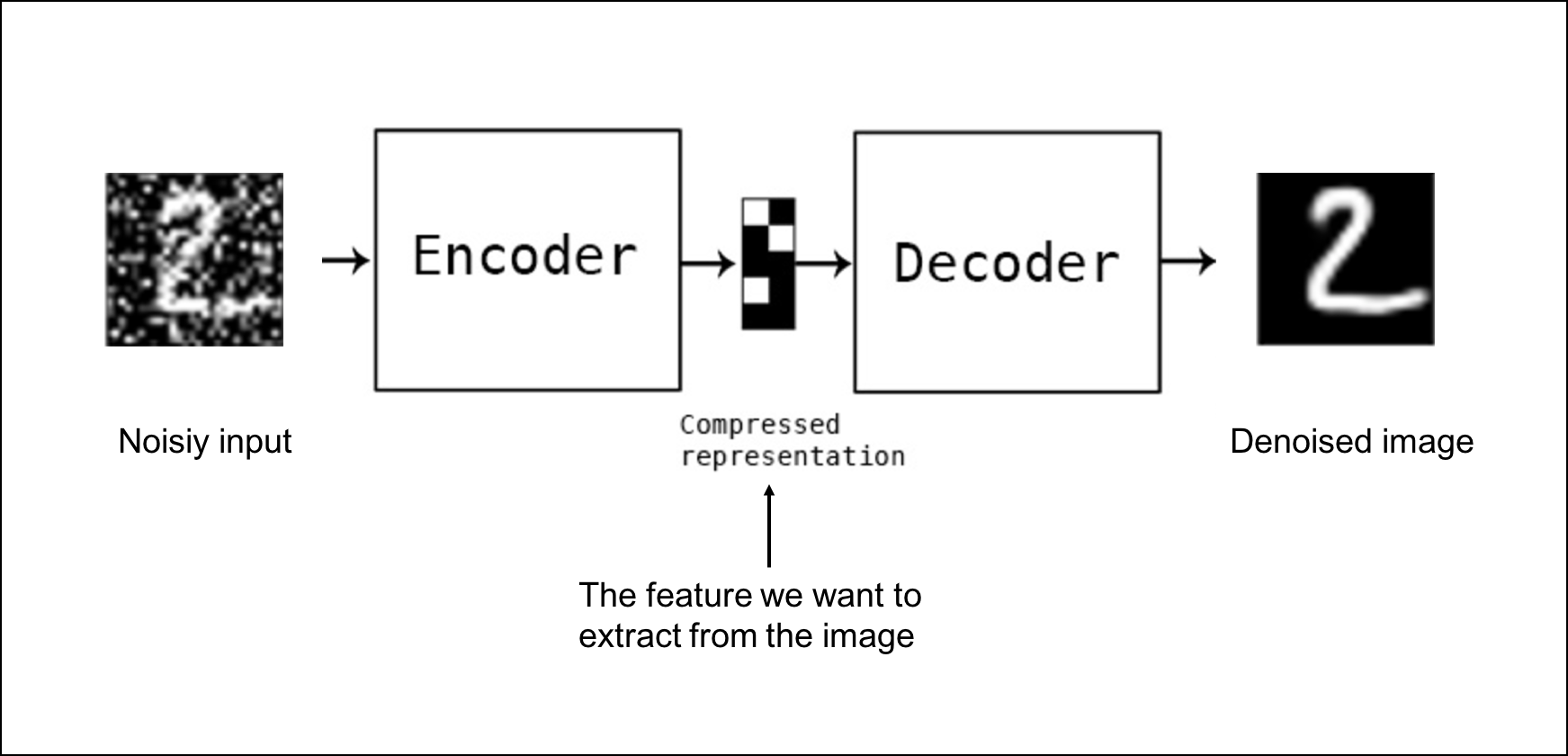
Understanding Autoencoders, GANs, and Diffusion Models – A Deep Dive

In this post, we’ll explore three key models in machine learning: Autoencoders, GANs (Generative Adversarial Networks), and Diffusion Models. These models, used for unsupervised learning, play a crucial role in tasks such as dimensionality reduction, feature extraction, and generating realistic data. We’ll look at how each model works, their architecture, and practical examples.

What Are Autoencoders?

Autoencoders are neural networks designed to compress input data into dense representations (known as latent representations) and then reconstruct it back to the original form. The goal is to minimize the difference between the input and the reconstructed data. This technique is extremely useful for:

• Dimensionality Reduction: Autoencoders help in reducing the dimensionality of high-dimensional data, while preserving the important features.
• Feature Extraction: They can act as feature detectors, helping with tasks like unsupervised learning or as part of a larger model.
• Generative Models: Autoencoders can generate new data that closely resemble the training data. For example, an autoencoder trained on face images can generate new face-like images.

Key Concepts in Autoencoders

Component	Description
Encoder	Compresses the input into a lower-dimensional representation.
Decoder	Reconstructs the original data from the compressed representation.
Reconstruction Loss	The difference between the original input and the output; minimized during training.

Link to Autoencoder Image to Understand Better (Copy and paste the link if it doesn’t open directly: https://www.analyticsvidhya.com/wp-content/uploads/2020/01/autoencoders)

In the image of the given above link , you can see the architecture of a simple autoencoder. The encoder compresses the input into a smaller representation, and the decoder tries to reconstruct it. The goal is to minimize the reconstruction loss.

Generative Adversarial Networks (GANs)

GANs take generative models to the next level. They consist of two neural networks:

1. Generator: The network that generates new data (e.g., synthetic images).
2. Discriminator: The network that evaluates the data, determining whether it is real or generated.

The generator and discriminator are in a constant battle. The generator tries to fool the discriminator by producing fake data, while the discriminator gets better at spotting fake data. This adversarial relationship helps improve both networks over time, resulting in highly realistic synthetic data.

How GANs Work:

1. The generator creates synthetic data.
2. The discriminator evaluates the data and determines if it’s real or fake.
3. The networks improve as they continue to challenge each other during training.

Component	Role
Generator	Creates fake data based on the training set.
Discriminator	Classifies data as real or fake.

Link to GAN Architecture Image to Understand Better (Copy and paste the link if it doesn’t open directly: https://developers.google.com/machine-learning/gan)

In the figure of the above given link, you see the adversarial relationship between the generator and discriminator. As the generator gets better at producing realistic data, the discriminator becomes more skilled at identifying fake data. This adversarial process leads to the generation of highly realistic synthetic data, making GANs a popular tool in AI art, video game graphics, and even deepfake videos.

Link to Explore GANs in Action (Generates Realistic Human Faces) (Copy and paste the link if it doesn’t open directly: https://thispersondoesnotexist.com)

This website showcases GANs in action, generating highly realistic human faces that don’t exist in reality.

Diffusion Models

A newer addition to the generative model family is the diffusion model. Introduced in 2021, these models generate more diverse and higher-quality images compared to GANs, but they are slower to train.

How Diffusion Models Work:

Diffusion models gradually add noise to an image, and then learn to remove that noise bit by bit. Essentially, the model learns how to denoise images, which can generate new images with higher quality over time.

Strength	Weakness
Produces higher-quality images	Slower to train
Easier to train than GANs

Link to Diffusion Model Image to Understand Better (Copy and paste the link if it doesn’t open directly: https://www.google.com/url?sa=t&source=web&rct=j&opi=89978449&url=https://colab.research.google.com/drive/1sjy9odlSSy0RBVgMTgP7s99NXsqglsUL%3Fusp%3Dsharing&ved=2ahUKEwjet5eyh6KJAxXXSPEDHR1LC4IQFnoECBQQAQ&usg=AOvVaw2I3IGWlh5DKlkjsPV4D1N)

This image demonstrates how noise is progressively added to an image during the diffusion process, and the model is trained to reverse this process, generating clean, high-quality images.

Real-world Application:

• Super-resolution: Diffusion models are often used to enhance the resolution of images.
• Creative Industries: These models are also applied in generative art and animation.

Comparison of Autoencoders, GANs, and Diffusion Models

Feature	Autoencoders	GANs	Diffusion Models
Training Type	Unsupervised	Adversarial (Unsupervised)	Unsupervised
Generative Capabilities	Limited (compared to GANs)	High-quality data generation	Higher quality than GANs but slower
Common Use Cases	Dimensionality reduction, noise removal	Synthetic data, image generation	Image denoising, super-resolution

A Practical Example of Implementing Autoencoders in TensorFlow

Autoencoders play a crucial role in machine learning for tasks like dimensionality reduction, data compression, and unsupervised pretraining. Let’s walk through an actual implementation in TensorFlow to illustrate their functionality.

Building a Simple Autoencoder

To begin, let’s construct a basic autoencoder. The architecture consists of two primary components: the encoder and the decoder. The encoder compresses the input into a lower-dimensional representation (latent space), while the decoder reconstructs the original input from this compressed representation.

import tensorflow as tf

encoder = tf.keras.Sequential([
    tf.keras.layers.Dense(2)
])

decoder = tf.keras.Sequential([
    tf.keras.layers.Dense(3)
])

autoencoder = tf.keras.Sequential([encoder, decoder])

optimizer = tf.keras.optimizers.SGD(learning_rate=0.5)
autoencoder.compile(loss="mse", optimizer=optimizer)

This autoencoder minimizes the reconstruction error using Mean Squared Error (MSE) loss and a Stochastic Gradient Descent (SGD) optimizer. The architecture is simple, consisting of a single layer for both the encoder and decoder.

Training the Autoencoder

Next, we train the autoencoder on a synthetic 3D dataset. In unsupervised learning tasks, the model is trained to reproduce its input. Therefore, the same data is used as both the input and the target.

X_train = [...]  # Generate a 3D dataset
history = autoencoder.fit(X_train, X_train, epochs=500, verbose=False)
codings = encoder.predict(X_train)

The model is trained for 500 epochs. After training, the encoder compresses the dataset into a lower-dimensional representation, effectively reducing its dimensionality.

Stacked Autoencoder for Dimensionality Reduction

For more complex data representation, we can stack multiple layers in both the encoder and decoder. This enables the autoencoder to learn more intricate patterns.

stacked_encoder = tf.keras.Sequential([
    tf.keras.layers.Flatten(),
    tf.keras.layers.Dense(100, activation="relu"),
    tf.keras.layers.Dense(30, activation="relu"),
])

stacked_decoder = tf.keras.Sequential([
    tf.keras.layers.Dense(100, activation="relu"),
    tf.keras.layers.Dense(28 * 28),
    tf.keras.layers.Reshape([28, 28])
])

stacked_ae = tf.keras.Sequential([stacked_encoder, stacked_decoder])
stacked_ae.compile(loss="mse", optimizer="nadam")

history = stacked_ae.fit(X_train, X_train, epochs=20, validation_data=(X_valid, X_valid))

Here, a stacked autoencoder with additional layers allows for better feature extraction. The Nadam optimizer enhances performance by combining momentum with adaptive learning rates.

Visualizing Reconstructions

After training, we can visualize how well the autoencoder reconstructs the input data, which helps determine if it has learned meaningful representations.

import numpy as np
import matplotlib.pyplot as plt

def plot_reconstructions(model, images=X_valid, n_images=5):
    reconstructions = np.clip(model.predict(images[:n_images]), 0, 1)

    fig = plt.figure(figsize=(n_images * 1.5, 3))
    for image_index in range(n_images):
        plt.subplot(2, n_images, 1 + image_index)
        plt.imshow(images[image_index], cmap="binary")
        plt.axis("off")
        plt.subplot(2, n_images, 1 + n_images + image_index)
        plt.imshow(reconstructions[image_index], cmap="binary")
        plt.axis("off")
    plt.show()

This function compares original validation images to their reconstructed versions, providing insights into the autoencoder’s performance.

Visualizing the Fashion MNIST Dataset

We can apply our stacked autoencoder to the Fashion MNIST dataset to reduce dimensionality and visualize the compressed data using t-SNE.

from sklearn.manifold import TSNE

X_valid_compressed = stacked_encoder.predict(X_valid)
tsne = TSNE(init="pca", learning_rate="auto", random_state=42)
X_valid_2D = tsne.fit_transform(X_valid_compressed)

plt.scatter(X_valid_2D[:, 0], X_valid_2D[:, 1], c=y_valid, s=10, cmap="tab10")
plt.show()

Here, we use the stacked encoder to reduce the dimensionality of the validation set. The t-SNE algorithm further reduces it to two dimensions for visualization, showing how well the autoencoder has captured the dataset’s variations.

Conclusion

Autoencoders, GANs, and diffusion models represent the cutting edge of generative AI, each offering unique capabilities to unlock the potential of data. Autoencoders excel at learning efficient representations, GANs push the boundaries of creativity by generating realistic data, and diffusion models introduce a powerful probabilistic framework for high-quality synthesis. Together, these technologies are reshaping industries, from art and entertainment to healthcare and beyond. As AI continues to evolve, understanding these models is no longer optional—it’s essential for anyone looking to stay ahead in the rapidly advancing world of machine learning. Embrace these tools, experiment with their possibilities, and unlock the secrets they hold to drive innovation and solve complex problems in ways we’ve only begun to imagine. The future of AI is here, and it’s waiting for you to explore.