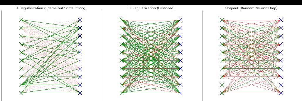
Understanding Regularization in Deep Learning

Understanding Regularization in Deep Learning – A Mathematical and Practical Approach

Introduction

One of the most compelling challenges in machine learning, particularly with deep learning models, is overfitting. This occurs when a model performs exceptionally well on the training data but fails to generalize to unseen data. Regularization offers solutions to this issue by controlling the complexity of the model and preventing it from overfitting. In this post, we’ll explore the different types of regularization techniques—L1, L2, and dropout—diving into their mathematical foundations and practical implementations.

What is Overfitting?

In machine learning, a model is said to be overfitting when it learns not just the actual patterns in the training data but also the noise and irrelevant details. While this enables the model to perform well on training data, it results in poor performance on new, unseen data.

The flexibility of neural networks, with their vast number of parameters, makes them highly prone to overfitting. This flexibility allows them to model very complex relationships in the data, but without precautions, they end up memorizing the training data instead of generalizing from it. Regularization is the key to addressing this challenge.

L1 and L2 Regularization: The Mathematical Backbone

L1 Regularization (Lasso Regression)

L1 regularization works by adding a penalty equal to the absolute value of the weights to the loss function. Mathematically, this is represented as:

$L_{L1} = L + \lambda \sum_{i} |\theta_i|$

Where:

$L$ is the original loss function (e.g., cross-entropy or mean squared error),
$\lambda$ is a regularization constant that controls the strength of regularization,
$\theta_i$ are the weights of the model.

L1 regularization promotes sparsity in the model. This means it forces many of the weights to zero, effectively removing certain features from the model. This can be useful when you expect that only a small subset of features will be significant for your task.

Why Use L1?

The reason L1 regularization is so useful in certain contexts is because it encourages the model to ignore irrelevant features. By forcing many of the weights to zero, it simplifies the model, making it more interpretable and preventing overfitting.

L2 Regularization (Ridge Regression or Weight Decay)

L2 regularization penalizes the squared values of the weights rather than the absolute values. The L2 regularized loss function is:

$L_{L2} = L + \lambda \sum_{i} \theta_i^2$

While L1 regularization forces some weights to zero, L2 regularization ensures that all the weights are small but not necessarily zero. This helps keep the model smooth and reduces overfitting without eliminating features entirely.

Why Use L2?

L2 regularization spreads the influence of all the input features more evenly, making it more suitable in cases where you expect all features to have some impact on the output. It’s the more commonly used regularization technique, particularly when the aim is to reduce overfitting without making the model sparse.

Dropout: A Different Approach

While L1 and L2 regularization modify the loss function, dropout takes a different approach. Introduced by Hinton et al., dropout randomly “drops” a certain percentage of neurons during training. By forcing the network to operate without certain neurons, dropout ensures that individual neurons don’t become too reliant on each other. This promotes robustness in the network and prevents overfitting.

Mathematically, dropout can be viewed as randomly setting the outputs of some neurons to zero with a probability $p$ . During testing, all neurons are used, but their activations are scaled down by $p$ to compensate for the missing neurons during training.

Why Use Dropout?

Dropout is particularly useful in deep neural networks, where overfitting is a common issue due to the high number of parameters. By introducing randomness, dropout ensures that the network cannot co-adapt too much to the training data, which helps generalize to unseen data.

How Regularization Works in Gradient Descent

In a typical training scenario, the model updates its weights using gradient descent. Without regularization, the update rule for weight $w$ is:

$w_{new} = w - \eta \frac{\partial L}{\partial w}$

Where:

$\eta$ is the learning rate,
$\frac{\partial L}{\partial w}$ is the gradient of the loss function with respect to $w$ .

With L2 regularization, the update rule changes to:

$w_{new} = w - \eta \left( \frac{\partial L}{\partial w} + \lambda w \right)$

This extra term $\lambda w$ penalizes large weights and shrinks them towards zero, effectively controlling the complexity of the model.

For L1 regularization, the update rule becomes:

$w_{new} = w - \eta \left( \frac{\partial L}{\partial w} + \lambda \cdot \text{sign}(w) \right)$

Here, $\text{sign}(w)$ is the sign of $w$ , which drives the weights toward zero for small values, promoting sparsity.

Practical Implementation: Regularization in Keras

In practice, implementing these regularization techniques is relatively straightforward in libraries like Keras. For example, applying L2 regularization to a dense layer is as simple as:


from tensorflow.keras import regularizers

model.add(Dense(64, kernel_regularizer=regularizers.l2(0.01)))

Similarly, you can apply dropout like this:


model.add(Dropout(0.5))

Here, 50% of the neurons will be dropped during each training iteration, making the network more robust.

TO NOTE NOW

Regularization is a critical tool for ensuring that deep learning models generalize well to unseen data. Whether it’s promoting sparsity through L1 regularization, shrinking weights through L2 regularization, or introducing randomness through dropout, each method has its strengths and can be used in various scenarios depending on the nature of the data and the model.

Incorporating these regularization techniques into your deep learning models can significantly improve their performance on new data, ensuring they don’t just memorize the training set but instead learn meaningful, generalizable patterns.

Aspect	L1 Regularization (Lasso)	L2 Regularization (Ridge)	Dropout	When to Use (Crystal Clear Use Case)
Penalty Term	Sum of the absolute values of the weights. $\lambda \sum \|w\|$	Sum of the squares of the weights. $\lambda \sum w^2$	No explicit penalty term, but neurons are randomly “dropped” during training, forcing the network to rely on different sets of neurons in each iteration.	How to Know Which One to Use: L1 Regularization (Lasso): Use when you suspect many features are irrelevant or redundant. L1 regularization is best suited for feature selection and sparse models. If you notice your model has many coefficients that are likely insignificant (especially in high-dimensional data), L1 will automatically drive some weights to zero, effectively eliminating irrelevant features. L2 Regularization (Ridge): Use when you believe all features contribute, but you want to prevent overfitting by reducing large weights. L2 regularization ensures all features contribute, but it minimizes the impact of each, controlling the magnitude. In datasets where multicollinearity (high correlation between variables) is an issue, L2 helps stabilize the model. Dropout: Use when working with deep neural networks, especially in fully connected layers, where overfitting is likely due to the high number of parameters. If your model shows signs of overfitting (e.g., the training accuracy is much higher than test accuracy), dropout can force the model to rely less on specific neurons, improving generalization. Mathematical Proof: L1: Minimizing the L1 penalty causes some weights to become zero, reducing the complexity of the model. This is seen in the optimization process where the gradient updates are smaller for irrelevant weights, eventually pushing them to zero: $w_{new} = w - \eta \left( \frac{\partial L}{\partial w} + \lambda \cdot \text{sign}(w) \right)$ . L2: The L2 penalty shrinks weights uniformly without eliminating any. This is effective when you want to reduce large weights but keep all features in the model: $w_{new} = w - \eta \left( \frac{\partial L}{\partial w} + \lambda w \right)$ . Dropout: By dropping neurons at random during training, the model learns to be more robust, generalizing better across datasets. The randomization forces the model to learn more distributed representations of the data.
Effect on Weights	Drives some weights to exactly zero, creating a sparse model by eliminating irrelevant features. $w_{new} = w - \eta \left( \frac{\partial L}{\partial w} + \lambda \cdot \text{sign}(w) \right)$	Reduces the magnitude of weights, but none are driven to exactly zero. Weights are shrunk by $\lambda w$ , but they never disappear. $w_{new} = w - \eta \left( \frac{\partial L}{\partial w} + \lambda w \right)$	Randomly “drops” neurons during training, zeroing their output temporarily to encourage the network to rely on different subsets of neurons.
Why Weights Go to Zero or Not	Weights go to zero because the penalty is based on the absolute value of the weights. This non-differentiability at zero means that the gradient can easily push small weights to zero, leading to sparsity.	Weights do not go to zero because the penalty is based on the square of the weights, which is differentiable everywhere. Weights are reduced in magnitude, but none are eliminated completely.	Weights are not permanently changed, but during training, some neurons are temporarily set to zero. This prevents the network from relying too much on any single set of neurons.
Computational Complexity	More complex, as L1 is not differentiable at zero, which can make optimization slower.	Less complex because L2 is differentiable everywhere, making optimization smoother.	Increases training time as the model needs more iterations to converge due to the random nature of dropout.
Example Scenario	In text classification, where only a small subset of words are predictive, L1 will drive irrelevant word features to zero, creating a sparse and interpretable model.	In regression models where multicollinearity is an issue, L2 regularization helps shrink all coefficients, making the model more stable without eliminating any feature.	In a deep neural network, dropout helps prevent overfitting by ensuring that the model does not rely too heavily on any one set of neurons, improving generalization.
Mathematical Example	For a linear regression problem with L1 regularization: $J(\theta) = \frac{1}{m} \sum_{i=1}^{m} (h_\theta (x^{(i)}) - y^{(i)})^2 + \lambda \sum \|\theta_j\|$ This drives irrelevant weights to zero, eliminating unnecessary features.	For a linear regression problem with L2 regularization: $J(\theta) = \frac{1}{m} \sum_{i=1}^{m} (h_\theta (x^{(i)}) - y^{(i)})^2 + \lambda \sum \theta_j^2$ This shrinks weights but doesn’t drive them to zero, keeping all features.	In a neural network with dropout, the output of neurons is zeroed out with probability $p$ . This prevents neurons from co-adapting during training.

Understanding L1 and L2 Regularization: A Numerical Proof

Wonder, Why Do Weights Go to Zero with L1 Regularization but Not with L2 Regularization? Lets do in this part a Numerical Proof with Multiple Iterations to know why

In machine learning, understanding why L1 regularization drives some weights to zero while L2 regularization does not is critical when choosing a regularization technique for your model. In this part, we will walk through multiple iterations of weight updates using both L1 and L2 regularization to show how L1 leads to sparsity (weights going to zero) while L2 shrinks weights but keeps them non-zero.

Overview of L1 and L2 Regularization

L1 Regularization (Lasso): Adds a penalty based on the absolute value of the weights. This often results in some weights being driven to zero, effectively removing irrelevant features and making the model sparse.
L2 Regularization (Ridge): Adds a penalty based on the square of the weights. This shrinks weights uniformly but never reduces them to zero, meaning all features continue to contribute to the model.

Mathematical Background: Why L1 Drives Weights to Zero and L2 Does Not

L1 Regularization

The cost function for L1 regularization is:

$J_{L1}(\theta) = \frac{1}{m} \sum_{i=1}^{m} (h_\theta(x^{(i)}) - y^{(i)})^2 + \lambda \sum |\theta_j|$

The key term is $|\theta_j|$ , the absolute value of the weights. Since the absolute value is non-differentiable at zero, small weights are often pushed all the way to zero during optimization. This leads to sparsity, where irrelevant features are discarded.

L2 Regularization

The cost function for L2 regularization is:

$J_{L2}(\theta) = \frac{1}{m} \sum_{i=1}^{m} (h_\theta(x^{(i)}) - y^{(i)})^2 + \lambda \sum \theta_j^2$

The key term is $\theta_j^2$ , the square of the weights. Since the square function is differentiable everywhere, it causes weights to shrink gradually but not reach zero. This maintains the contribution of all features, though their influence is reduced.

Numerical Example: Multiple Iterations of L1 and L2 Regularization

Let’s walk through a numerical example, applying both L1 and L2 regularization to show how the weights evolve over multiple iterations of gradient descent.

Assumptions

We have two weights: $\theta_1 = 1.5$ and $\theta_2 = 0.5$ .
Regularization strength $\lambda = 0.1$ .
Learning rate $\eta = 0.1$ .
Assume a simple gradient $\frac{\partial L}{\partial \theta} = 1$ for both weights.

Without Regularization

In the absence of regularization, the weights remain unchanged by the regularization penalty.

Initial weights:

theta_1 = 1.5
theta_2 = 0.5

After one iteration of gradient descent (assuming the gradient $\frac{\partial L}{\partial \theta} = 1$ ):

theta_1 = 1.5 - 0.1 * 1 = 1.4
theta_2 = 0.5 - 0.1 * 1 = 0.4

This continues for more iterations, but the weights are simply reduced by the learning rate multiplied by the gradient without any additional penalty.

L1 Regularization (Iteration by Iteration)

Let’s see what happens to the weights when L1 regularization is applied over several iterations.

Iteration 1

theta_1 = 1.5 - 0.1 * (1 + 0.1 * sign(1.5)) = 1.5 - 0.11 = 1.39
theta_2 = 0.5 - 0.1 * (1 + 0.1 * sign(0.5)) = 0.5 - 0.11 = 0.39

Iteration 2

theta_1 = 1.39 - 0.1 * (1 + 0.1 * sign(1.39)) = 1.39 - 0.11 = 1.28
theta_2 = 0.39 - 0.1 * (1 + 0.1 * sign(0.39)) = 0.39 - 0.11 = 0.28

Iteration 3

theta_1 = 1.28 - 0.1 * (1 + 0.1 * sign(1.28)) = 1.28 - 0.11 = 1.17
theta_2 = 0.28 - 0.1 * (1 + 0.1 * sign(0.28)) = 0.28 - 0.11 = 0.17

Iteration 4

theta_1 = 1.17 - 0.1 * (1 + 0.1 * sign(1.17)) = 1.17 - 0.11 = 1.06
theta_2 = 0.17 - 0.1 * (1 + 0.1 * sign(0.17)) = 0.17 - 0.11 = 0.06

Iteration 5

theta_1 = 1.06 - 0.1 * (1 + 0.1 * sign(1.06)) = 1.06 - 0.11 = 0.95
theta_2 = 0.06 - 0.1 * (1 + 0.1 * sign(0.06)) = 0.06 - 0.11 = 0  # pushed to zero

In subsequent iterations, $\theta_2$ will remain at zero, and $\theta_1$ will continue to decrease gradually.

L2 Regularization (Iteration by Iteration)

Now let’s see what happens with L2 regularization over several iterations.

Iteration 1

theta_1 = 1.5 - 0.1 * (1 + 0.1 * 1.5) = 1.5 - 0.115 = 1.385
theta_2 = 0.5 - 0.1 * (1 + 0.1 * 0.5) = 0.5 - 0.105 = 0.395

Iteration 2

theta_1 = 1.385 - 0.1 * (1 + 0.1 * 1.385) = 1.385 - 0.11385 = 1.27115
theta_2 = 0.395 - 0.1 * (1 + 0.1 * 0.395) = 0.395 - 0.10395 = 0.29105

Iteration 3

theta_1 = 1.27115 - 0.1 * (1 + 0.1 * 1.27115) = 1.27115 - 0.1127 = 1.15845
theta_2 = 0.29105 - 0.1 * (1 + 0.1 * 0.29105) = 0.29105 - 0.10291 = 0.18814

Iteration 4

theta_1 = 1.15845 - 0.1 * (1 + 0.1 * 1.15845) = 1.15845 - 0.11158 = 1.04687
theta_2 = 0.18814 - 0.1 * (1 + 0.1 * 0.18814) = 0.18814 - 0.10188 = 0.08626

Iteration 5

theta_1 = 1.04687 - 0.1 * (1 + 0.1 * 1.04687) = 1.04687 - 0.11047 = 0.93640
theta_2 = 0.08626 - 0.1 * (1 + 0.1 * 0.08626) = 0.08626 - 0.10086 = -0.0146

As you can see, in L2 regularization, the weights continuously shrink but do not reach zero. The penalty on the square of the weights forces them to get smaller, but never eliminates any weight completely.

TO NOTE NOW

L1 Regularization causes weights to go to zero because the penalty is based on the absolute value of the weights, which is not differentiable at zero. This makes L1 regularization ideal for feature selection and creating sparse models, where many weights will become exactly zero.

L2 Regularization, on the other hand, reduces weights but does not make any of them zero. It shrinks the weights uniformly, which is useful when you want to control overfitting but keep all features in the model.

In summary, use L1 Regularization when you need feature selection or a sparse model, and use L2 Regularization when you want to shrink weights without eliminating any features.

What is Dropout Regularization ? /title><br /> <style id="wpr-lazyload-bg-container"></style><style id="wpr-lazyload-bg-exclusion"></style> <noscript> <style id="wpr-lazyload-bg-nostyle">.page-title-default{--wpr-bg-ed2268f8-3ab3-40f5-a757-4fffecc624fb: url('https://ingoampt.com/wp-content/uploads/2021/09/shoes-page-title.jpg');}.page-title-default{--wpr-bg-f6447a2a-5688-48b5-8213-5b98e73d384d: url('https://ingoampt.com/wp-content/uploads/2021/09/shoes-page-title.jpg');}.rll-youtube-player .play{--wpr-bg-fbb3b65f-22c2-4f7f-9f60-812b6246d6f8: url('https://ingoampt.com/wp-content/plugins/wp-rocket/assets/img/youtube.png');}</style> </noscript> <script type="application/javascript">const rocket_pairs = [{"selector":".page-title-default","style":".page-title-default{--wpr-bg-ed2268f8-3ab3-40f5-a757-4fffecc624fb: url('https:\/\/ingoampt.com\/wp-content\/uploads\/2021\/09\/shoes-page-title.jpg');}","hash":"ed2268f8-3ab3-40f5-a757-4fffecc624fb","url":"https:\/\/ingoampt.com\/wp-content\/uploads\/2021\/09\/shoes-page-title.jpg"},{"selector":".page-title-default","style":".page-title-default{--wpr-bg-f6447a2a-5688-48b5-8213-5b98e73d384d: url('https:\/\/ingoampt.com\/wp-content\/uploads\/2021\/09\/shoes-page-title.jpg');}","hash":"f6447a2a-5688-48b5-8213-5b98e73d384d","url":"https:\/\/ingoampt.com\/wp-content\/uploads\/2021\/09\/shoes-page-title.jpg"},{"selector":".rll-youtube-player .play","style":".rll-youtube-player .play{--wpr-bg-fbb3b65f-22c2-4f7f-9f60-812b6246d6f8: url('https:\/\/ingoampt.com\/wp-content\/plugins\/wp-rocket\/assets\/img\/youtube.png');}","hash":"fbb3b65f-22c2-4f7f-9f60-812b6246d6f8","url":"https:\/\/ingoampt.com\/wp-content\/plugins\/wp-rocket\/assets\/img\/youtube.png"}]; const rocket_excluded_pairs = [];</script></head><br /> <body></p> <p>Note : L2 regularization is particularly effective when using traditional optimizers like <strong>SGD (Stochastic Gradient Descent)</strong>, <strong>momentum optimization</strong>, and <strong>Nesterov momentum</strong>. However, it doesn’t pair well with the <strong>Adam optimizer</strong>, which uses adaptive learning rates. Instead of using traditional L2 regularization, <strong>AdamW</strong> is the preferred variant when applying weight decay with the Adam optimizer. AdamW decouples weight decay from the learning rate adaptation, ensuring that weight decay is applied correctly while maintaining Adam’s learning rate benefits.</p> <h4>Key Takeaway:</h4> <ul> <li><strong>Use L2 Regularization</strong> when you need to penalize large weights and encourage the model to generalize better. If using the Adam optimizer, switch to <strong>AdamW</strong> to handle weight decay effectively.</li> </ul> <hr> <h2>Exploring Dropout Regularization</h2> <p><strong>Dropout</strong> is a different kind of regularization technique that combats overfitting by randomly dropping a subset of neurons during each training iteration. This forces the remaining neurons to step up, ensuring that the model does not become overly reliant on specific neurons. The result is a more generalized and robust model, as the network learns redundant representations that make it more resistant to noise in the data.</p> <h3>How Dropout Works</h3> <p>During training, each neuron has a probability $ p $ of being “dropped” or turned off. This means that the neuron is temporarily excluded from both the forward and backward passes during that iteration of training. Typical values for the <strong>dropout rate</strong> range from 10%-50%, depending on the type of neural network architecture:</p> <ul> <li>In <strong>recurrent neural networks (RNNs)</strong>, dropout rates typically range between <strong>20% and 30%</strong>.</li> <li>In <strong>convolutional neural networks (CNNs)</strong>, dropout rates are generally higher, often ranging from <strong>40% to 50%</strong>.</li> </ul> <p>Once training is complete, dropout is turned off during inference, meaning that all neurons are active, but their outputs are scaled to account for the dropout that occurred during training. This ensures that the model’s predictions remain stable and accurate.</p> <h3>Why Dropout Works</h3> <p>Dropout ensures that the neurons in the network do not rely too heavily on any specific input or neighbor neurons. Each neuron has to “learn” to function effectively on its own, creating a network that generalizes better to new data. This makes dropout an effective regularization technique, especially in deep neural networks where overfitting is a significant concern.</p> <h4>Key Takeaway:</h4> <ul> <li><strong>Use Dropout</strong> when training deep networks to prevent overfitting, especially if your model has a lot of parameters and you notice it performing too well on training data but poorly on validation data. Adjust the dropout rate depending on your architecture (20%-30% for RNNs, 40%-50% for CNNs).</li> </ul> <hr> <h2>An Interesting Analogy for Dropout</h2> <p>To understand dropout better, Imagine a company where employees are randomly told each morning whether or not they should go to work. The company would be forced to adapt, as the employees who do show up must perform tasks that others would typically handle. Over time, this would create a more resilient organization because employees would become more versatile, learning to perform various tasks and not relying solely on a few individuals.</p> <p>Similarly, in a neural network, dropout forces neurons to adapt by distributing the learning across the network. No single neuron can dominate the learning process, making the network more flexible and less prone to overfitting.</p> <hr> <h4>Key Takeaway:</h4> <ul> <li><strong>Dropout</strong> helps distribute learning across neurons, preventing any single neuron from becoming too critical for the network’s performance. This enhances the model’s ability to generalize to new, unseen examples.</li> </ul> <p><!DOCTYPE html><br /> <html lang="en"><br /> <head><br /> <br /> <meta name="viewport" content="width=device-width, initial-scale=1.0"><br /> <title>Practical Code Implementation for L2 Regularization and Dropout

Practical Code Implementation for L2 Regularization and Dropout in TensorFlow/Keras, PyTorch, and MLX

In the previous section, we discussed the theory behind L2 regularization and dropout. Now, let’s dive into how you can implement these techniques in popular deep learning frameworks: TensorFlow/Keras, PyTorch, and MLX (Apple Silicon’s optimized machine learning framework).

1. TensorFlow/Keras Example

L2 Regularization in TensorFlow/Keras

In TensorFlow/Keras, L2 regularization can be applied using the kernel_regularizer argument in layers like Dense. Here’s an example:


import tensorflow as tf
from tensorflow.keras import layers, regularizers

# Define a simple Sequential model with L2 regularization
model = tf.keras.Sequential([
    layers.Dense(128, activation='relu', kernel_regularizer=regularizers.l2(0.01)),
    layers.Dense(64, activation='relu', kernel_regularizer=regularizers.l2(0.01)),
    layers.Dense(10, activation='softmax')  # Output layer for classification
])

# Compile the model
model.compile(optimizer='adam',
              loss='sparse_categorical_crossentropy',
              metrics=['accuracy'])

# Train the model
model.fit(X_train, y_train, epochs=10, validation_data=(X_val, y_val))

Dropout in TensorFlow/Keras

Adding dropout layers to your Keras model is easy. Use the Dropout layer to randomly drop neurons during training.


import tensorflow as tf
from tensorflow.keras import layers

# Define a model with dropout regularization
model = tf.keras.Sequential([
    layers.Dense(128, activation='relu'),
    layers.Dropout(0.5),  # Dropout with 50% probability
    layers.Dense(64, activation='relu'),
    layers.Dropout(0.5),  # Another Dropout layer
    layers.Dense(10, activation='softmax')  # Output layer for classification
])

# Compile the model
model.compile(optimizer='adam',
              loss='sparse_categorical_crossentropy',
              metrics=['accuracy'])

# Train the model
model.fit(X_train, y_train, epochs=10, validation_data=(X_val, y_val))

2. PyTorch Example

L2 Regularization in PyTorch

In PyTorch, L2 regularization (also called weight decay) is set via the weight_decay argument in the optimizer.


import torch
import torch.nn as nn
import torch.optim as optim

# Define a simple neural network with PyTorch
class Net(nn.Module):
    def __init__(self):
        super(Net, self).__init__()
        self.fc1 = nn.Linear(784, 128)
        self.fc2 = nn.Linear(128, 64)
        self.fc3 = nn.Linear(64, 10)
    
    def forward(self, x):
        x = torch.relu(self.fc1(x))
        x = torch.relu(self.fc2(x))
        x = self.fc3(x)
        return x

# Initialize the network
model = Net()

# Use AdamW optimizer with L2 regularization (weight decay)
optimizer = optim.AdamW(model.parameters(), lr=0.001, weight_decay=0.01)  # L2 regularization

# Loss function
criterion = nn.CrossEntropyLoss()

# Training loop (simplified)
for epoch in range(10):
    for data, target in train_loader:
        optimizer.zero_grad()
        output = model(data)
        loss = criterion(output, target)
        loss.backward()
        optimizer.step()

Dropout in PyTorch

Dropout can be added using the nn.Dropout layer in PyTorch. Here’s how you can implement it:


import torch
import torch.nn as nn
import torch.optim as optim

# Define a neural network with dropout
class Net(nn.Module):
    def __init__(self):
        super(Net, self).__init__()
        self.fc1 = nn.Linear(784, 128)
        self.drop1 = nn.Dropout(0.5)  # 50% dropout
        self.fc2 = nn.Linear(128, 64)
        self.drop2 = nn.Dropout(0.5)  # Another dropout
        self.fc3 = nn.Linear(64, 10)
    
    def forward(self, x):
        x = torch.relu(self.fc1(x))
        x = self.drop1(x)  # Apply dropout
        x = torch.relu(self.fc2(x))
        x = self.drop2(x)  # Apply dropout
        x = self.fc3(x)
        return x

# Initialize the model
model = Net()

# Optimizer and loss
optimizer = optim.Adam(model.parameters(), lr=0.001)
criterion = nn.CrossEntropyLoss()

# Training loop (simplified)
for epoch in range(10):
    for data, target in train_loader:
        optimizer.zero_grad()
        output = model(data)
        loss = criterion(output, target)
        loss.backward()
        optimizer.step()

3. MLX (Apple Silicon) Example

L2 Regularization and Dropout in MLX

Apple’s MLX framework is optimized for Apple Silicon hardware. Here’s how you can apply L2 regularization and dropout in an MLX model:


import mlx
from mlx import nn, optim

# Define a neural network model in MLX
model = nn.Sequential(
    nn.Linear(784, 128),
    nn.ReLU(),
    nn.Dropout(0.5),  # Dropout layer with 50% probability
    nn.Linear(128, 64),
    nn.ReLU(),
    nn.Dropout(0.5),  # Another dropout layer
    nn.Linear(64, 10)
)

# Set up an optimizer with L2 regularization (weight decay)
optimizer = optim.AdamW(model.parameters(), lr=0.001, weight_decay=0.01)  # L2 regularization

# Training loop (simplified)
for epoch in range(10):
    for data, target in train_loader:
        optimizer.zero_grad()
        output = model(data)
        loss = nn.CrossEntropyLoss(output, target)
        loss.backward()
        optimizer.step()

In this example:

Dropout layers are added between the fully connected layers.
L2 regularization is applied using the weight_decay argument in the AdamW optimizer.

Apple Silicon’s unified memory architecture allows for efficient memory sharing between the CPU and GPU, making the computations more efficient.

Difference Between Dropout and L1 Regularization

Aspect	L1 Regularization	Dropout
What is affected	Model weights (encourages weights to become zero)	Neurons/units (temporarily drops neurons during training)
Mathematical effect	Adds penalty term to loss based on absolute weight values	Randomly disables neurons, but doesn’t change weights directly
Use case	Useful for sparse models and feature selection	Effective for deep learning to prevent co-adaptation of neurons
Effect on model	Simplifies the model by shrinking some weights to zero	Forces the model to distribute learning across all neurons
Training impact	Gradually removes unimportant weights permanently	Temporarily removes neurons during training, not permanently
Inference	Sparse model with fewer weights	All neurons active during inference, no dropout applied

Conclusion

In this post, we have implemented L1 and L2 regularization and dropout using three different machine learning frameworks: TensorFlow/Keras, PyTorch, and MLX. These regularization techniques are essential for reducing overfitting and building models that generalize well to unseen data. Depending on the framework and hardware you’re using, you can choose the right tools to apply these techniques effectively.

Education

Understanding Regularization in Deep Learning – day 47

Understanding Regularization in Deep Learning – A Mathematical and Practical Approach

Introduction

What is Overfitting?

L1 and L2 Regularization: The Mathematical Backbone

L1 Regularization (Lasso Regression)

Why Use L1?

L2 Regularization (Ridge Regression or Weight Decay)

Why Use L2?

Dropout: A Different Approach

Why Use Dropout?

How Regularization Works in Gradient Descent

Practical Implementation: Regularization in Keras

TO NOTE NOW

Wonder, Why Do Weights Go to Zero with L1 Regularization but Not with L2 Regularization? Lets do in this part a Numerical Proof with Multiple Iterations to know why

Overview of L1 and L2 Regularization

Mathematical Background: Why L1 Drives Weights to Zero and L2 Does Not

L1 Regularization

L2 Regularization

Numerical Example: Multiple Iterations of L1 and L2 Regularization

Assumptions

Without Regularization

L1 Regularization (Iteration by Iteration)

Iteration 1

Iteration 2

Iteration 3

Iteration 4

Iteration 5

L2 Regularization (Iteration by Iteration)

Iteration 1

Iteration 2

Iteration 3

Iteration 4

Iteration 5

TO NOTE NOW

Practical Code Implementation for L2 Regularization and Dropout in TensorFlow/Keras, PyTorch, and MLX

1. TensorFlow/Keras Example

L2 Regularization in TensorFlow/Keras

Dropout in TensorFlow/Keras

2. PyTorch Example

L2 Regularization in PyTorch

Dropout in PyTorch

3. MLX (Apple Silicon) Example

L2 Regularization and Dropout in MLX

Difference Between Dropout and L1 Regularization

Conclusion

don't miss our new posts. Subscribe for updates

Related Posts

Privacy Policies

Quick Links