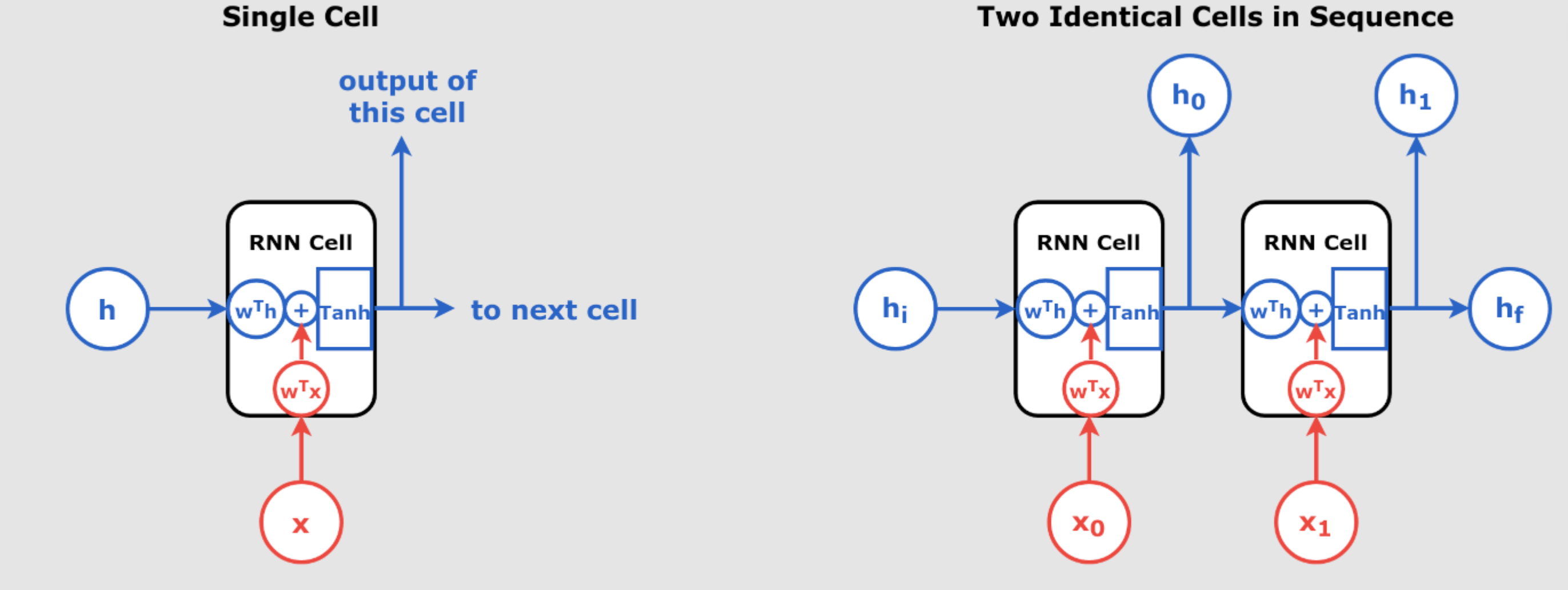
Understanding Recurrent Neural Networks (RNNs) – part 2 – day 56

September 26, 2024
Posted by ingoampt

Understanding Recurrent Neural Networks (RNNs): A Deep Dive into Sequential Learning

Recurrent Neural Networks (RNNs) are a class of neural networks that excel in handling sequential data, such as time series, text, and speech. Unlike traditional feedforward networks, RNNs have the ability to retain information from previous inputs and use it to influence the current output, making them extremely powerful for tasks where the order of the input data matters.

In this article, we will explore the inner workings of RNNs, break down their key components, and understand how they process sequences of data through time. We’ll also dive into how they are trained using Backpropagation Through Time (BPTT) and explore different types of sequence processing architectures like Sequence-to-Sequence and Encoder-Decoder Networks.

What is a Recurrent Neural Network (RNN)?

At its core, an RNN is a type of neural network that introduces the concept of “memory” into the model. Each neuron in an RNN has a feedback loop that allows it to use both the current input and the previous output to make decisions. This creates a temporal dependency, enabling the network to learn from past information.

Recurrent Neuron: The Foundation of RNNs

A recurrent neuron processes sequences by not only considering the current input but also the output from the previous time step. This memory feature allows RNNs to preserve information over time, making them ideal for handling sequential data.

In mathematical terms, a single recurrent neuron at time t receives:

X(t), the input vector at time t
ŷ(t-1), the output vector from the previous time step

The output of a recurrent neuron at time t is computed as:

$\hat{y}(t) = \phi (W_x^T X(t) + W_y \hat{y}(t-1) + b)$

Where:

$W_x$ is the weight matrix applied to the input at time $t$
$W_y$ is the weight matrix applied to the previous output
$\phi$ is an activation function (e.g., ReLU or sigmoid)
$b$ is a bias term

This equation illustrates how the output at any given time step depends not only on the current input but also on the outputs of previous time steps, allowing the network to “remember” past information.

Unrolling Through Time

To train an RNN, the recurrent neuron can be unrolled through time, meaning that we treat each time step as a separate layer in a neural network. Each layer passes its output to the next one. By unrolling the network, we can visualize how RNNs handle sequences step-by-step.

For example, if a sequence $X = [X(0), X(1), X(2), X(3)]$ is fed into the network, the recurrent neuron produces a sequence of outputs $\hat{y} = [\hat{y}(0), \hat{y}(1), \hat{y}(2), \hat{y}(3)]$ , with each output influenced by both the current input and previous outputs.

Layers of Recurrent Neurons

In practical applications, we often stack multiple recurrent neurons to form a layer. In this case, the inputs and outputs become vectors, and the network maintains two sets of weights:

$W_x$ , connecting the inputs at time $t$
$W_y$ , connecting the previous outputs

The output for a layer of recurrent neurons in a mini-batch is computed as:

$\hat{Y}(t) = \phi (X(t) W_x + \hat{Y}(t-1) W_y + b)$

Where:

$X(t)$ is the input at time step $t$
$\hat{Y}(t-1)$ is the output from the previous time step
$W_x$ and $W_y$ are weight matrices
$b$ is a bias vector

Memory Cells: A Step Toward Long-Term Dependencies

While simple RNNs are capable of learning short-term dependencies, they often struggle to capture longer-term patterns in data. To address this limitation, more advanced RNN architectures introduce Memory Cells like Long Short-Term Memory (LSTM) networks and Gated Recurrent Units (GRUs).

In these architectures, the network maintains a hidden state $h(t)$ at time step $t$ , which is a function of both the current input and the previous hidden state:

$h(t) = f(X(t), h(t-1))$

This hidden state serves as a memory that can retain relevant information for many time steps, allowing the network to capture long-term dependencies in sequential data.

Sequence-to-Sequence and Encoder-Decoder Networks

RNNs are highly versatile and can be used in various architectures to solve different tasks. Here are some common RNN architectures:

Sequence-to-Sequence Networks

In a Sequence-to-Sequence network, the model takes a sequence of inputs and produces a sequence of outputs. For example, this type of network could be used for machine translation, where the input is a sequence of words in one language, and the output is the translation in another language.

Sequence-to-Vector Networks

In a Sequence-to-Vector network, the model processes a sequence of inputs but only produces a single output at the end. This architecture is often used for sentiment analysis, where the network processes an entire sentence (a sequence) and outputs a single sentiment score.

Vector-to-Sequence Networks

In a Vector-to-Sequence network, the input is a single vector, and the output is a sequence. A common example of this architecture is generating captions for images, where the input is an image vector, and the output is a sequence of words.

Encoder-Decoder Networks

An Encoder-Decoder network is a two-step process where the Encoder converts the input sequence into a single vector, and the Decoder generates the output sequence. This architecture is commonly used in tasks like machine translation, where the input and output sequences are of different lengths.

Training RNNs with Backpropagation Through Time (BPTT)

Training RNNs is more complex than training feedforward networks because of the temporal dependencies in the data. To train an RNN, we use a process called Backpropagation Through Time (BPTT).

Feature	Backpropagation (Feedforward Networks)	Backpropagation Through Time (BPTT) (RNNs)
Network Type	Feedforward Neural Networks (FNNs)	Recurrent Neural Networks (RNNs)
Data Type	Fixed-size, non-sequential data	Sequential data (e.g., time-series, text)
Unrolling	No unrolling, single forward/backward pass	Unrolled across time steps (treated like deep layers)
Dependencies	No temporal dependencies	Temporal dependencies, where each time step depends on previous steps
Gradient Calculation	Gradients are calculated layer by layer	Gradients are backpropagated through each time step and summed
Weight Sharing	Weights are unique to each layer	Weights are shared across time steps
Memory Usage	Lower memory, as only layers are involved	Higher memory due to storing multiple time steps
Vanishing/Exploding Gradients	Less frequent (still possible in deep networks)	More common due to long sequences (mitigated by techniques like gradient clipping)
Applications	Image classification, basic regression	Time-series prediction, language modeling, speech recognition
Loss Calculation	Loss is computed after a single forward pass	Loss is computed at each time step, and summed over the sequence
Challenges	Simple gradient flow	Gradient flow through multiple time steps can lead to issues like vanishing gradients

Unrolling for Training

During training, the RNN is “unrolled” through multiple time steps. The output at each time step is compared to the target output, and the loss is computed for the entire sequence. This loss is then propagated backward through the unrolled network to update the weights using gradient descent.

Loss Function

In a sequence-to-sequence task, for example, we might only care about the final output. In this case, the loss is computed based on the last output, and the gradients are propagated backward through the unrolled network, but only the relevant outputs are used to compute the gradients.

For instance, the loss might be computed as:

$\mathcal{L}(Y(2), Y(3), Y(4), \hat{Y}(2), \hat{Y}(3), \hat{Y}(4))$

Where $Y(t)$ represents the true output and $\hat{Y}(t)$ is the predicted output at time $t$ .

Conclusion: The Power of RNNs in Sequential Learning

Recurrent Neural Networks are a powerful tool for learning from sequential data. Whether it’s for time series prediction, text generation, or machine translation, RNNs enable models to capture patterns in data that extend beyond individual input points. While training these networks can be more complex than traditional feedforward networks, techniques like Backpropagation Through Time ensure that they learn efficiently from temporal data.

Moreover, advanced architectures like LSTMs and Encoder-Decoder Networks allow RNNs to handle more complex tasks by introducing memory cells and multi-step processing. As we continue to advance in the field of deep learning, RNNs and their variants will remain a cornerstone for tasks that require learning from sequential and temporal data.

By understanding the inner workings of RNNs, we open the door to solving a wide range of problems where sequence matters, from speech recognition to natural language processing.

Education