Announcement : Ai academy : deep learning
Enhance your deep learning journey with the AI Academy: Deep Learning app, designed to simplify complex AI concepts through interactive flashcards and personalized notes. Whether […]
Enhance your deep learning journey with the AI Academy: Deep Learning app, designed to simplify complex AI concepts through interactive flashcards and personalized notes. Whether […]
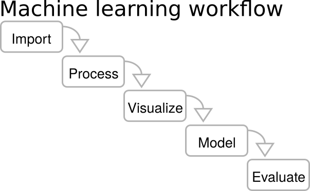
Where to Get Data for Machine Learning and Deep Learning Model Creation Where to Get Data for Machine Learning and Deep Learning Model Creation 1. […]
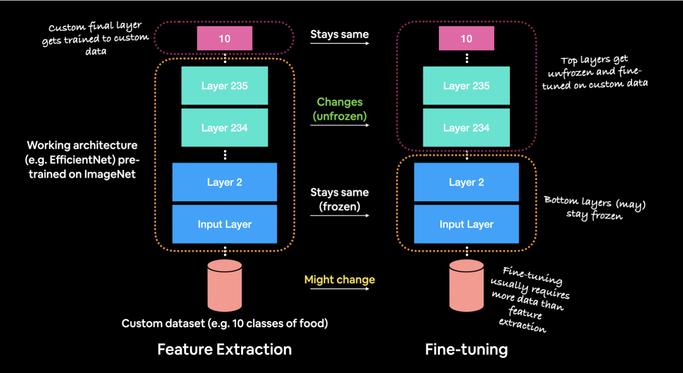
Understanding Fine-Tuning in Deep Learning Understanding Fine-Tuning in Deep Learning: A Comprehensive Overview Fine-tuning in deep learning has become a powerful technique, allowing developers to […]
What is NLP and the Math Behind It? Understanding Transformers and Deep Learning in NLP Introduction to NLP Natural Language Processing (NLP) is a crucial subfield of artificial intelligence (AI) that focuses on enabling machines to process and understand human language. Whether it’s machine translation, chatbots, or text analysis, NLP helps bridge the gap between human communication and machine understanding. But what’s behind NLP’s ability to understand and generate language? Underneath it all lies sophisticated mathematics and cutting-edge models like deep learning and transformers. This post will delve into the fundamentals of NLP, the mathematical principles that power it, and...
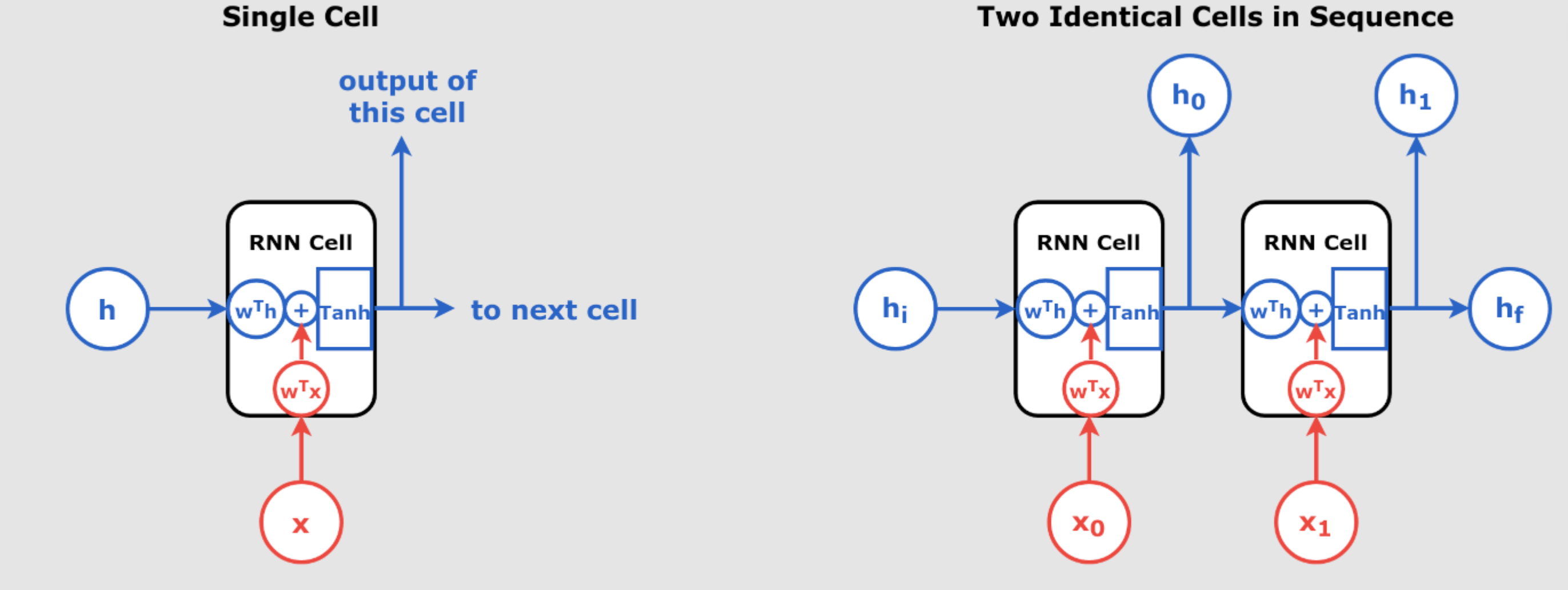
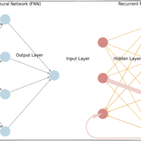
Understanding Recurrent Neural Networks (RNNs) Recurrent Neural Networks (RNNs) are a class of neural networks that excel in handling sequential data, such as time series, text, and speech. Unlike traditional feedforward networks, RNNs have the ability to retain information from previous inputs and use it to influence the current output, making them extremely powerful for tasks where the order of the input data matters. In day 55 article we have introduced RNN. In this article, we will explore the inner workings of RNNs, break down their key components, and understand how they process sequences of data through time. We’ll also...
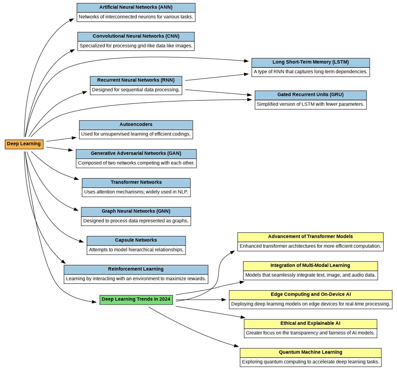
Key Deep Learning Models for iOS Apps Natural Language Processing (NLP) Models NLP models enable apps to understand and generate human-like text, supporting features like chatbots, sentiment analysis, and real-time translation. Top NLP Models for iOS: • Transformers (e.g., GPT, BERT, T5): Powerful for text generation, summarization, and answering queries. • Llama: A lightweight, open-source alternative to GPT, ideal for mobile apps due to its resource efficiency. Example Use Cases: • Building chatbots with real-time conversational capabilities. • Developing sentiment analysis tools for analyzing customer feedback. • Designing language translation apps for global users. Integration Tools: • Hugging Face: Access...
Understanding Dropout in Neural Networks with a Real Numerical Example In deep learning, overfitting is a common problem where a model performs extremely well on training data but fails to generalize to unseen data. One popular solution is dropout, which randomly deactivates neurons during training, making the model more robust. In this section, we will demonstrate dropout with a simple example using numbers and explain how dropout manages weights during training. What is Dropout? Dropout is a regularization technique used in neural networks to prevent overfitting. In a neural network, neurons are connected between layers, and dropout randomly turns off...
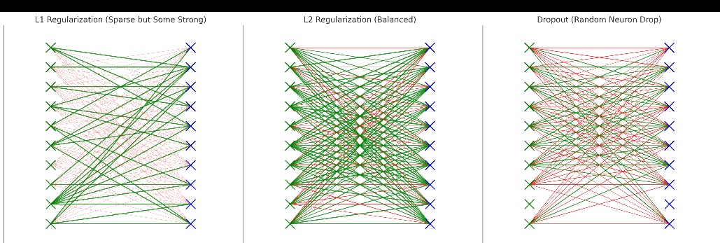
Understanding Regularization in Deep Learning – A Mathematical and Practical Approach Introduction One of the most compelling challenges in machine learning, particularly with deep learning models, is overfitting. This occurs when a model performs exceptionally well on the training data but fails to generalize to unseen data. Regularization offers solutions to this issue by controlling the complexity of the model and preventing it from overfitting. In this post, we’ll explore the different types of regularization techniques—L1, L2, and dropout—diving into their mathematical foundations and practical implementations. What is Overfitting? In machine learning, a model is said to be overfitting when...
Advanced Learning Rate Scheduling Methods for Machine Learning: Learning rate scheduling is critical in optimizing machine learning models, helping them converge faster and avoid pitfalls such as getting stuck in local minima. So far in our pervious days articles we have explained a lot about optimizers, learning rate schedules, etc. In this guide, we explore three key learning rate schedules: Exponential Decay, Cyclic Exponential Decay (CED), and 1-Cycle Scheduling, providing mathematical proofs, code implementations, and theory behind each method. 1. Exponential Decay Learning Rate Exponential Decay reduces the learning rate by a factor of , allowing larger updates early in...

The 1Cycle Learning Rate Policy: Accelerating Model Training In our pervious article (day 42) , we have explained The Power of Learning Rates in Deep Learning and Why Schedules Matter, lets now focus on 1Cycle Learning Rate to explain it in more detail : The 1Cycle Learning Rate Policy, first introduced by Leslie Smith in 2018, remains one of the most effective techniques for optimizing model training. By 2025, it continues to prove its efficiency, accelerating convergence by up to 10x compared to traditional learning rate schedules, such as constant or exponentially decaying rates. Today, both researchers and practitioners...
For best results, phrase your question similar to our FAQ examples.