RNN Deep Learning – Part 1 – Day 55

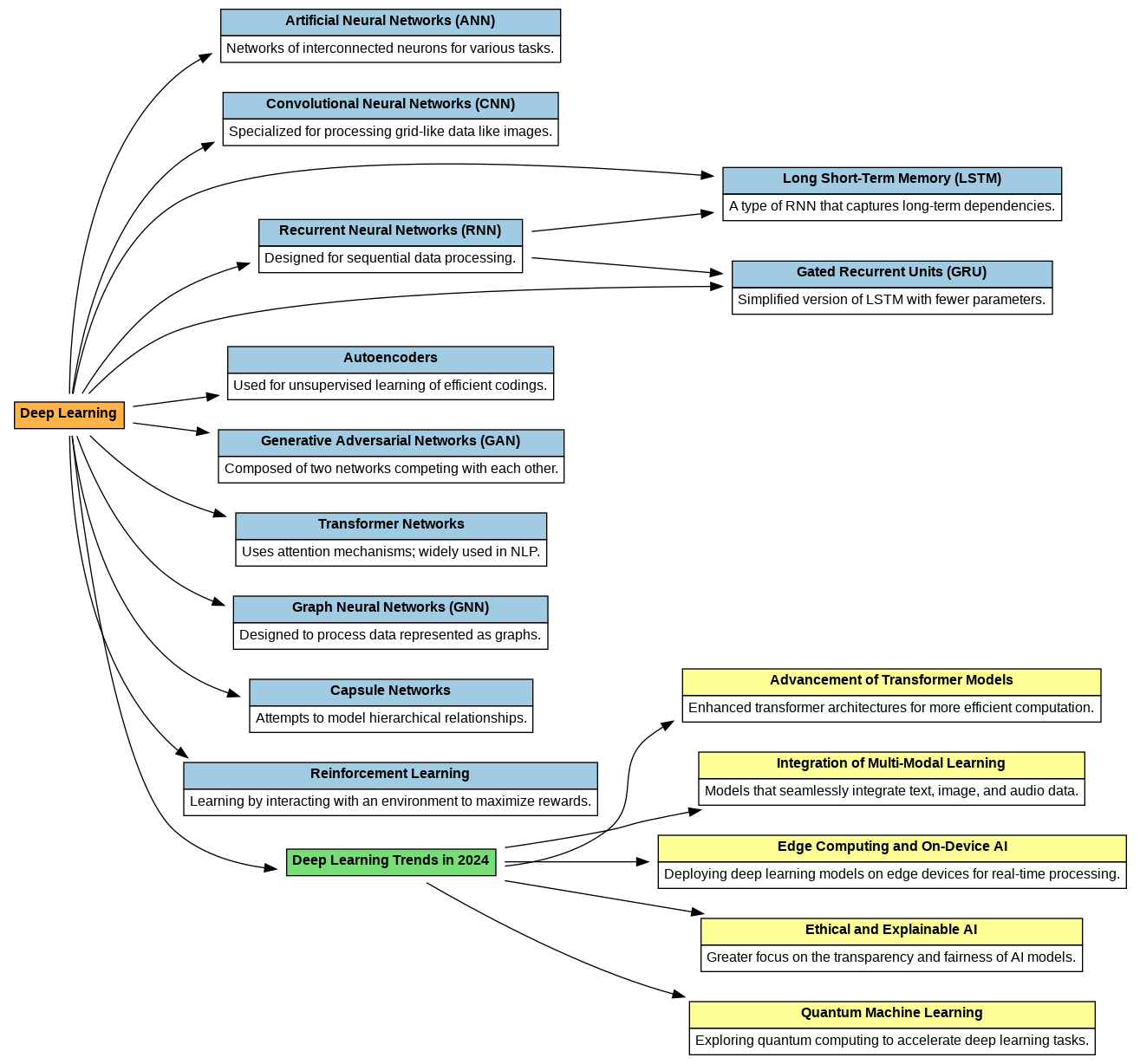
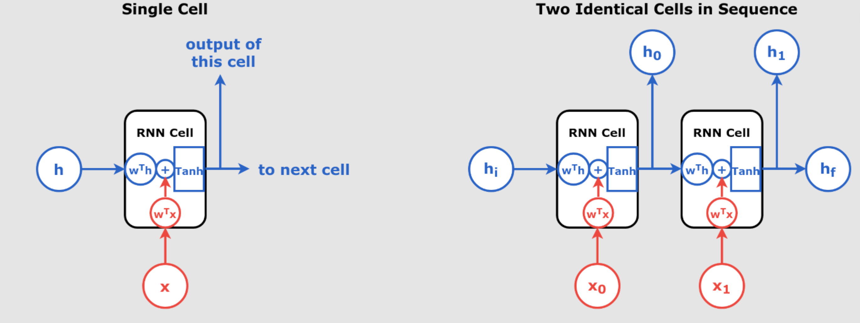
Understanding Recurrent Neural Networks (RNNs) and CNNs for Sequence Processing Introduction In the world of deep learning, neural networks have become indispensable, especially for handling tasks involving sequential data, such as time series, speech, and text. Among the most popular architectures for such data are Recurrent Neural Networks (RNNs) and Convolutional Neural Networks (CNNs). Although RNNs are traditionally associated with sequence processing, CNNs have also been adapted to perform well in this area. This blog will take a detailed look at how these networks work, their differences, their challenges, and their real-world applications.  Unrolling RNNs: How RNNs Process Sequences One of the most important concepts in understanding RNNs is unrolling. Unlike feedforward neural networks, which process inputs independently, RNNs have a “memory” that allows them to keep track of previous inputs by maintaining hidden states. Unrolling in Time At each time step \( t \), an RNN processes both: The current input \( x(t) \) The hidden state \( h(t-1) \), which contains information from the previous steps The RNN essentially performs the same task repeatedly at each step, but it does so by incorporating past data (via the hidden state), making it ideal for sequence data. Time Step Input...

Membership Required

You must be a member to access this content.

View Membership Levels

Already a member? Log in here

Deep Learning Models integration for iOS Apps – briefly explained – Day 52

Key Deep Learning Models for iOS Apps Natural Language Processing (NLP) Models NLP models enable apps to understand and generate human-like text, supporting features like chatbots, sentiment analysis, and real-time translation. Top NLP Models for iOS: • Transformers (e.g., GPT, BERT, T5): Powerful for text generation, summarization, and answering queries. • Llama: A lightweight, open-source alternative to GPT, ideal for mobile apps due to its resource efficiency. Example Use Cases: • Building chatbots with real-time conversational capabilities. • Developing sentiment analysis tools for analyzing customer feedback. • Designing language translation apps for global users. Integration Tools: • Hugging Face: Access pre-trained models like GPT, BERT, and Llama for immediate integration. • PyTorch: Fine-tune models and convert them to Core ML for iOS deployment. Generative AI Models Generative AI models create unique content, including text, images, and audio, making them crucial for creative apps. Top Generative AI Models: • GANs (Generative Adversarial Networks): Generate photorealistic images, videos, and audio. • Llama with Multimodal Extensions: Handles both text and images efficiently, ideal for creative applications. • VAEs (Variational Autoencoders): Useful for reconstructing data and personalization. Example Use Cases: • Apps for generating digital art and music. • Tools for personalized content creation,...

Membership Required

You must be a member to access this content.

View Membership Levels

Already a member? Log in here

DropOut and Monte Carlo Dropout (MC Dropout)- Day 48

Understanding Dropout in Neural Networks Understanding Dropout in Neural Networks with a Real Numerical Example In deep learning, overfitting is a common problem where a model performs extremely well on training data but fails to generalize to unseen data. One popular solution is dropout, which randomly deactivates neurons during training, making the model more robust. In this section, we will demonstrate dropout with a simple example using numbers and explain how dropout manages weights during training. What is Dropout? Dropout is a regularization technique used in neural networks to prevent overfitting. In a neural network, neurons are connected between layers, and dropout randomly turns off a subset of those neurons during the training phase. When dropout is applied, each neuron has a probability \( p \) of being “dropped out” (i.e., set to zero). For instance, if \( p = 0.5 \), each neuron has a 50% chance of being dropped for a particular training iteration. Importantly, dropout does not remove neurons or weights permanently. Instead, it temporarily deactivates them during training, and they may be active again in future iterations.   Let’s walk through a numerical example to see how dropout works in action and how weights are managed...

Membership Required

You must be a member to access this content.

View Membership Levels

Already a member? Log in here

Understanding Regularization in Deep Learning – Day 47

Understanding Regularization in Deep Learning – A Mathematical and Practical Approach Introduction One of the most compelling challenges in machine learning, particularly with deep learning models, is overfitting. This occurs when a model performs exceptionally well on the training data but fails to generalize to unseen data. Regularization offers solutions to this issue by controlling the complexity of the model and preventing it from overfitting. In this post, we’ll explore the different types of regularization techniques—L1, L2, and dropout—diving into their mathematical foundations and practical implementations. What is Overfitting? In machine learning, a model is said to be overfitting when it learns not just the actual patterns in the training data but also the noise and irrelevant details. While this enables the model to perform well on training data, it results in poor performance on new, unseen data. The flexibility of neural networks, with their vast number of parameters, makes them highly prone to overfitting. This flexibility allows them to model very complex relationships in the data, but without precautions, they end up memorizing the training data instead of generalizing from it. Regularization is the key to addressing this challenge. L1 and L2 Regularization: The Mathematical Backbone L1 Regularization (Lasso...

Membership Required

You must be a member to access this content.

View Membership Levels

Already a member? Log in here

Learning Rate – 1-Cycle Scheduling, exponential decay and Cyclic Exponential Decay (CED) – Part 4 – Day 45

Advanced Learning Rate Scheduling Methods for Machine Learning: Learning rate scheduling is critical in optimizing machine learning models, helping them converge faster and avoid pitfalls such as getting stuck in local minima. So far in our pervious days articles we have explained a lot about optimizers, learning rate schedules, etc. In this guide, we explore three key learning rate schedules: Exponential Decay, Cyclic Exponential Decay (CED), and 1-Cycle Scheduling, providing mathematical proofs, code implementations, and theory behind each method. 1. Exponential Decay Learning Rate Exponential Decay reduces the learning rate by a factor of , allowing larger updates early in training and smaller, more refined updates as the model approaches convergence. Formula: Where: is the learning rate at time step , is the initial learning rate, is the decay rate, controlling how fast the learning rate decreases, represents the current time step (or epoch). Mathematical Proof of Exponential Decay The core idea of exponential decay is that the learning rate decreases over time. Let’s prove that this results in convergence. The parameter update rule for gradient descent is: Substituting the exponentially decayed learning rate: As , the decay factor , meaning that the updates to become smaller and smaller, allowing...

Membership Required

You must be a member to access this content.

View Membership Levels

Already a member? Log in here
landscape photography of mountains covered in snow

Theory Behind 1Cycle Learning Rate Scheduling & Learning Rate Schedules – Day 43

  The 1Cycle Learning Rate Policy: Accelerating Model Training  In our pervious article  (day 42) , we have explained The Power of Learning Rates in Deep Learning and Why Schedules Matter, lets now focus on 1Cycle Learning Rate to explain it  in more detail :  The 1Cycle Learning Rate Policy, first introduced by Leslie Smith in 2018, remains one of the most effective techniques for optimizing model training. By 2025, it continues to prove its efficiency, accelerating convergence by up to 10x compared to traditional learning rate schedules, such as constant or exponentially decaying rates. Today, both researchers and practitioners are pushing the boundaries of deep learning with this method, solidifying its role as a key component in the training of modern AI models. How the 1Cycle Policy Works The 1Cycle policy deviates from conventional learning rate schedules by alternating between two distinct phases: Phase 1: Increasing Learning Rate – The learning rate starts low and steadily rises to a peak value (η_max). This phase promotes rapid exploration of the loss landscape, avoiding sharp local minima. Phase 2: Decreasing Learning Rate – Once the peak is reached, the learning rate gradually decreases to a very low value, enabling the model...

Membership Required

You must be a member to access this content.

View Membership Levels

Already a member? Log in here

The Power of Learning Rates in Deep Learning and Why Schedules Matter – Day 42

  The Power of Learning Rates in Deep Learning and Why Schedules Matter In deep learning, one of the most critical yet often overlooked hyperparameters is the learning rate. It dictates how quickly a model updates its parameters during training, and finding the right learning rate can make the difference between a highly effective model and one that never converges. This post delves into the intricacies of learning rates, their sensitivity, and how to fine-tune training using learning rate schedules. Why is Learning Rate Important? The learning rate controls the size of the step the optimizer takes when adjusting model parameters during each iteration of training. If this step is too large, the model may overshoot the optimal values and fail to converge, leading to oscillations in the loss function. On the other hand, a very small learning rate causes training to proceed too slowly, taking many epochs to approach the global minimum. Learning Rate Sensitivity Here’s what happens with different learning rates: Too High: With a high learning rate, the model may diverge entirely, with the loss function increasing rapidly due to overshooting. This can cause the model to fail entirely. Too Low: A low learning rate leads to...

Membership Required

You must be a member to access this content.

View Membership Levels

Already a member? Log in here

Adam vs SGD vs AdaGrad vs RMSprop vs AdamW – Day 39

Choosing the Best Optimizer for Your Deep Learning Model When training deep learning models, choosing the right optimization algorithm can significantly impact your model’s performance, convergence speed, and generalization ability. Below, we will explore some of the most popular optimization algorithms, their strengths, the reasons they were invented, and the types of problems they are best suited for. 1. Stochastic Gradient Descent (SGD) Why It Was Invented SGD is one of the earliest and most fundamental optimization algorithms used in machine learning and deep learning. It was invented to handle the challenge of minimizing cost functions efficiently, particularly when dealing with large datasets where traditional gradient descent methods would be computationally expensive. Inventor The concept of SGD is rooted in statistical learning, but its application in neural networks is often attributed to Yann LeCun and others in the 1990s. Formula The update rule for SGD is given by: where is the learning rate, is the gradient of the loss function with respect to the model parameters . Strengths and Limitations **Strengths:** SGD is particularly effective in cases where the model is simple, and the dataset is large, making it a robust choice for problems where generalization is important. The simplicity...

Membership Required

You must be a member to access this content.

View Membership Levels

Already a member? Log in here

AdaGrad vs RMSProp vs Adam: Why Adam is the Most Popular? – Day 38

A Comprehensive Guide to Optimization Algorithms: AdaGrad, RMSProp, and Adam In the realm of machine learning, selecting the right optimization algorithm can significantly impact the performance and efficiency of your models. Among the various options available, AdaGrad, RMSProp, and Adam are some of the most widely used optimization algorithms. Each of these algorithms has its own strengths and weaknesses. In this article, we’ll explore why AdaGrad ( which we explained fully on day 37 ) might not always be the best choice and how RMSProp & Adam could address some of its shortcomings. AdaGrad: Why It’s Not Always the Best Choice What is AdaGrad? AdaGrad (Adaptive Gradient Algorithm) is one of the first adaptive learning rate methods. It adjusts the learning rate for each parameter individually by scaling it inversely with the sum of the squares of all previous gradients. The Core Idea: The idea behind AdaGrad is to use a different learning rate for each parameter that adapts over time based on the historical gradients. Parameters with large gradients will have their learning rates decreased, while parameters with small gradients will have their learning rates increased. The Core Equation: Where: represents the parameters at time step . is the...

Membership Required

You must be a member to access this content.

View Membership Levels

Already a member? Log in here

Nag as optimiser in deep learning – day 36

Nesterov Accelerated Gradient (NAG): A Comprehensive Overview Nesterov Accelerated Gradient (NAG): A Comprehensive Overview Introduction to Nesterov Accelerated Gradient Nesterov Accelerated Gradient (NAG), also known as Nesterov Momentum, is an advanced optimization technique introduced by Yurii Nesterov in the early 1980s. It is an enhancement of the traditional momentum-based optimization used in gradient descent, designed to accelerate the convergence rate of the optimization process, particularly in the context of deep learning and complex optimization problems. How NAG Works The core idea behind NAG is the introduction of a “look-ahead” step before calculating the gradient, which allows for a more accurate and responsive update of parameters. In traditional momentum methods, the gradient is computed at the current position of the parameters, which might lead to less efficient convergence if the trajectory is not perfectly aligned with the optimal path. NAG, however, calculates the gradient at a position slightly ahead, based on the accumulated momentum, thus allowing the algorithm to “correct” its course more effectively if it is heading towards a suboptimal direction. The NAG update rule can be summarized as follows: Look-ahead Step: Compute a preliminary update based on the momentum. Gradient Calculation: Evaluate the gradient at this look-ahead position. Momentum...

Membership Required

You must be a member to access this content.

View Membership Levels

Already a member? Log in here