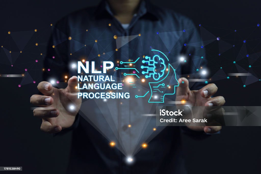
Introduction to Natural Language Processing (NLP)

Natural Language Processing (NLP) has always been at the cutting edge of AI, enabling machines to interpret and generate human language. With the rapid development of deep learning models and large language models (LLMs) like GPT and BERT, NLP has seen transformative changes. As we move into 2024, advancements such as emotional recognition, better handling of unstructured data, and the rise of modular architectures are expected to drive the field forward.

From improving chatbots to facilitating multilingual processing, NLP plays a vital role in industries ranging from customer service to healthcare. But it’s the combination of Recurrent Neural Networks (RNNs), attention mechanisms, and cutting-edge Transformer models that truly shapes the future of NLP.

RNNs in NLP: A Powerful Tool for Sequential Data

Recurrent Neural Networks (RNNs) are a key architecture for handling sequential data, making them highly suitable for NLP tasks. They have the ability to “remember” past inputs, which is crucial when processing sentences where the meaning of each word depends on its context. For instance, when generating text, an RNN uses previously generated words to predict the next one.

Character-Level RNNs (Char-RNN)

Char-RNNs are a fascinating example of how RNNs work in text generation. These models generate text one character at a time, predicting the next character based on the ones before it. A char-RNN trained on Shakespeare’s works, for instance, will generate new text that mimics Shakespeare’s style, showing how effectively RNNs can capture and reproduce the nuances of language. However, RNNs alone often struggle with long-term dependencies, which is why more advanced models like GRUs and LSTMs were introduced to handle these issues more efficiently.

Source: Predibase

Stateful vs. Stateless RNNs

• Stateless RNNs process each sequence independently, resetting their hidden states after each batch, which is effective for short sequences but struggles with long-term context.
• Stateful RNNs, on the other hand, retain their hidden state across batches, making them more suited for long sequences, where maintaining the context is essential for making accurate predictions.

The Evolution to Attention Mechanisms and Transformers

While RNNs were the cornerstone of NLP in earlier years, the introduction of attention mechanisms revolutionized the field. These mechanisms enable models to focus on the most relevant parts of an input sequence, which significantly improved performance in complex tasks like machine translation and text summarization.

Transformer architectures, like BERT and GPT, further advanced the field by allowing parallel processing of input data. Transformers leverage self-attention, which enables them to consider all words in a sentence at once, making them more efficient than RNNs, which process data sequentially. By 2024, Transformers are expected to dominate NLP research and application, outpacing RNNs in many areas due to their scalability and efficiency.

Source: DATAVERSITY

What’s New in NLP for 2024 and Beyond?

1. Localized Large Language Models (LLMs): By 2025, we expect to see a shift towards localized LLMs, such as Llama2, which are preferred over centralized models like ChatGPT due to security concerns and the ability to integrate industry-specific knowledge. These models will allow businesses to customize AI solutions for their unique contexts, making them a better fit for industries like healthcare, finance, and law.
2. Combinational AI and LangChain: New technologies like LangChain allow combining the outputs of different LLMs to solve more complex, multi-step problems. This “combinational AI” approach enables the integration of models that understand user intent, detect sentiment, and generate responses—all working in harmony to provide deeper insights.
3. Emotion and Sentiment Recognition: NLP is evolving to handle not just the semantics of language, but also its emotional undertones. Models are becoming adept at detecting sentiment in customer interactions, allowing businesses to respond with more empathy and improve customer experience.
4. Hybrid and Neuroscience-based Models: Hybrid models, which combine different architectures like RNNs and CNNs (Convolutional Neural Networks), are gaining popularity for their ability to capture both spatial and temporal dependencies in data. Additionally, neuroscience-inspired models are emerging, drawing from the workings of the human brain to create more sophisticated, human-like learning algorithms.
5. Explainable and Ethical AI: With the growing deployment of AI in critical applications, ensuring transparency and fairness has become a major focus. Efforts to create explainable AI (XAI) models that provide insights into their decision-making processes will play a key role in industries where biased decisions can have serious consequences, such as finance and healthcare.
6. Modular Architectures and Synthetic Data: In 2024, we’ll see the rise of modular architectures in large language models, allowing for more flexible and scalable solutions. Additionally, synthetic data is becoming increasingly common for training AI models, offering an alternative to expensive and privacy-sensitive real-world datasets. This shift is helping models achieve higher performance with smaller, highly curated datasets.

Source: Predibase

Key Takeaways

• RNNs remain important for sequence modeling tasks, but Transformers and attention mechanisms are proving more efficient for many NLP applications.
• Localized LLMs, combinational AI, and neuroscience-based models are driving the next wave of NLP advancements in 2024.
• Ethical considerations and transparency are critical as NLP is integrated into industries like finance, healthcare, and customer service.
• Modular architectures and the use of synthetic data are becoming essential for creating scalable and explainable AI systems.

Introduction

So far, we have discussed the theoretical foundation behind Recurrent Neural Networks (RNNs) and their applications in Natural Language Processing (NLP). Now, we’ll bring those concepts to life by implementing a character-level RNN (char-RNN) to generate Shakespearean text. Each part of the code is tied to the key stages of RNN-based deep learning, and we’ll explain the rationale behind each choice.

Step 1: Data Loading and Preprocessing (Preprocessing Stage)

The first step in any deep learning model is data preparation. For RNNs, this means transforming raw text data into a form that can be processed by the network.

import tensorflow as tf

shakespeare_url = "https://homl.info/shakespeare"  # shortcut URL
filepath = tf.keras.utils.get_file("shakespeare.txt", shakespeare_url)
with open(filepath) as f:
    shakespeare_text = f.read()

Explanation and Connection to RNN Training Stages:
Data Preprocessing is a crucial stage in deep learning. For RNNs, especially in NLP, this involves preparing sequential data so that each character or word is properly represented. This stage is common to all types of neural networks but particularly important for RNNs because they process data step by step over time, so every detail in the text (characters in this case) matters.

Step 2: Text Vectorization (Input Encoding)

Before feeding the text into the RNN, it must be transformed into numerical format. This process is known as vectorization.

text_vec_layer = tf.keras.layers.TextVectorization(
    split="character",  # character-level encoding
    standardize="lower"  # convert to lowercase to reduce complexity
)
text_vec_layer.adapt([shakespeare_text])
encoded = text_vec_layer([shakespeare_text])[0].numpy()  # Convert to numpy array

Explanation and Connection to RNN Training Stages:
Input Encoding: The RNN needs data in numerical format, as it can’t process raw text. By vectorizing the text at the character level, we ensure that each character is represented by an integer. The TextVectorization layer converts text into a format suitable for processing by an RNN. This step is crucial for sequence models like RNNs, where each element in the sequence (character) must be properly represented so the network can learn temporal dependencies.

Step 3: Preparing Data for the RNN (Training Data Setup)

Now, we prepare overlapping sequences from the encoded text. These sequences are used to train the RNN to predict the next character in a sequence.

encoded -= 2  # Drop tokens 0 (pad) and 1 (unknown)
n_tokens = text_vec_layer.vocabulary_size() - 2
dataset_size = len(encoded)

def to_dataset(sequence, length, shuffle=False, seed=None, batch_size=32):
    ds = tf.data.Dataset.from_tensor_slices(sequence)
    ds = ds.window(length + 1, shift=1, drop_remainder=True)
    ds = ds.flat_map(lambda window_ds: window_ds.batch(length + 1))
    if shuffle:
        ds = ds.shuffle(buffer_size=100_000, seed=seed)
    ds = ds.batch(batch_size)
    return ds.map(lambda window: (window[:, :-1], window[:, 1:])).prefetch(1)

Explanation and Connection to RNN Training Stages:
Training Data Setup: RNNs are trained on sequences, and here we are generating sliding windows of input-target pairs. Each window is a sequence of characters, where the RNN learns to predict the next character in the sequence. The RNN needs sequential data because it builds an internal “memory” of the previous inputs to predict the next output. Preparing the data in this way allows the network to learn these temporal dependencies.

Step 4: Splitting the Dataset (Training/Validation/Test Split)

We split the dataset into training, validation, and test sets.

length = 100
tf.random.set_seed(42)
train_set = to_dataset(encoded[:1_000_000], length=length, shuffle=True, seed=42)
valid_set = to_dataset(encoded[1_000_000:1_060_000], length=length)
test_set = to_dataset(encoded[1_060_000:], length=length)

Explanation and Connection to RNN Training Stages:
Training/Validation/Test Split: This step ensures the model’s performance is validated and tested on unseen data. The RNN learns from the training set, while the validation set ensures it generalizes well during training. The test set is used to evaluate final performance after training. Splitting the data helps prevent overfitting, which is especially important for sequence models like RNNs that can memorize sequences too well without generalizing properly.

Step 5: Building the Char-RNN Model (Model Definition)

We define the RNN architecture, specifying the type of RNN we’ll use (GRU) and adding an embedding layer and a dense output layer.

model = tf.keras.Sequential([
    tf.keras.layers.Embedding(input_dim=n_tokens, output_dim=16),
    tf.keras.layers.GRU(128, return_sequences=True),
    tf.keras.layers.Dense(n_tokens, activation="softmax")
])

model.compile(loss="sparse_categorical_crossentropy", optimizer="nadam", metrics=["accuracy"])

model_ckpt = tf.keras.callbacks.ModelCheckpoint(
    "my_shakespeare_model", monitor="val_accuracy", save_best_only=True
)

Explanation and Connection to RNN Training Stages:
Model Definition: We use an Embedding layer to convert integer character IDs into dense vectors. The GRU layer processes the sequence, and the Dense layer outputs the predicted next character.
Why GRU? We are using a GRU (Gated Recurrent Unit) because it is a simpler and faster variant of an LSTM (Long Short-Term Memory) but still effectively manages long-term dependencies. GRUs control the flow of information using gates, making them ideal for tasks where long-range dependencies need to be captured (such as text generation).

Step 6: Training the Model (Model Training)

We train the model using the training data, validating performance at each epoch.

history = model.fit(train_set, validation_data=valid_set, epochs=10, callbacks=[model_ckpt])

Explanation and Connection to RNN Training Stages:
Model Training: This step involves feeding the sequential data into the RNN, which adjusts its weights through backpropagation based on the loss function (sparse categorical crossentropy in this case). Callbacks like ModelCheckpoint are used to save the best-performing version of the model during training. Training the RNN involves repeatedly presenting it with sequences and having it learn the temporal dependencies between characters.

Step 7: Making Predictions (Inference/Prediction)

Finally, after training the model, we can use it to generate text. Given a sequence, the model predicts the next character.

shakespeare_model = tf.keras.Sequential([
    text_vec_layer,
    tf.keras.layers.Lambda(lambda X: X - 2),  # subtract 2 from character IDs
    model
])

y_proba = shakespeare_model.predict(["To be or not to b"])[0, -1]
y_pred = tf.argmax(y_proba)
text_vec_layer.get_vocabulary()[y_pred + 2]

Explanation and Connection to RNN Training Stages:
Inference/Prediction: Once the model is trained, we use it for generating new text. We provide a seed sequence (e.g., “To be or not to b”) and predict the next character. This process can be repeated to generate longer sequences. Argmax is used to select the character with the highest probability, and the TextVectorization layer converts the predicted character ID back into a readable character. The Lambda layer adjusts for the padding tokens removed earlier.

RNN Type and Why We Use GRU

Why GRU? GRUs are chosen for this task because they strike a good balance between performance and complexity. Unlike basic RNNs, GRUs can maintain long-term dependencies, and they are computationally simpler than LSTMs, making them faster to train. For text generation tasks where long sequences of dependencies (like in Shakespearean text) need to be captured, GRUs offer an efficient solution without the risk of losing important context over time.

Conclusion

In this section, we walked through the steps to implement a char-RNN to generate text in Shakespeare’s style. By following the steps of preprocessing, model definition, training, and inference, we’ve seen how an RNN can be used to learn from sequential data and generate new text. The choice of GRU for this task helps to efficiently manage long-term dependencies and generate coherent, Shakespearean-style sequences.