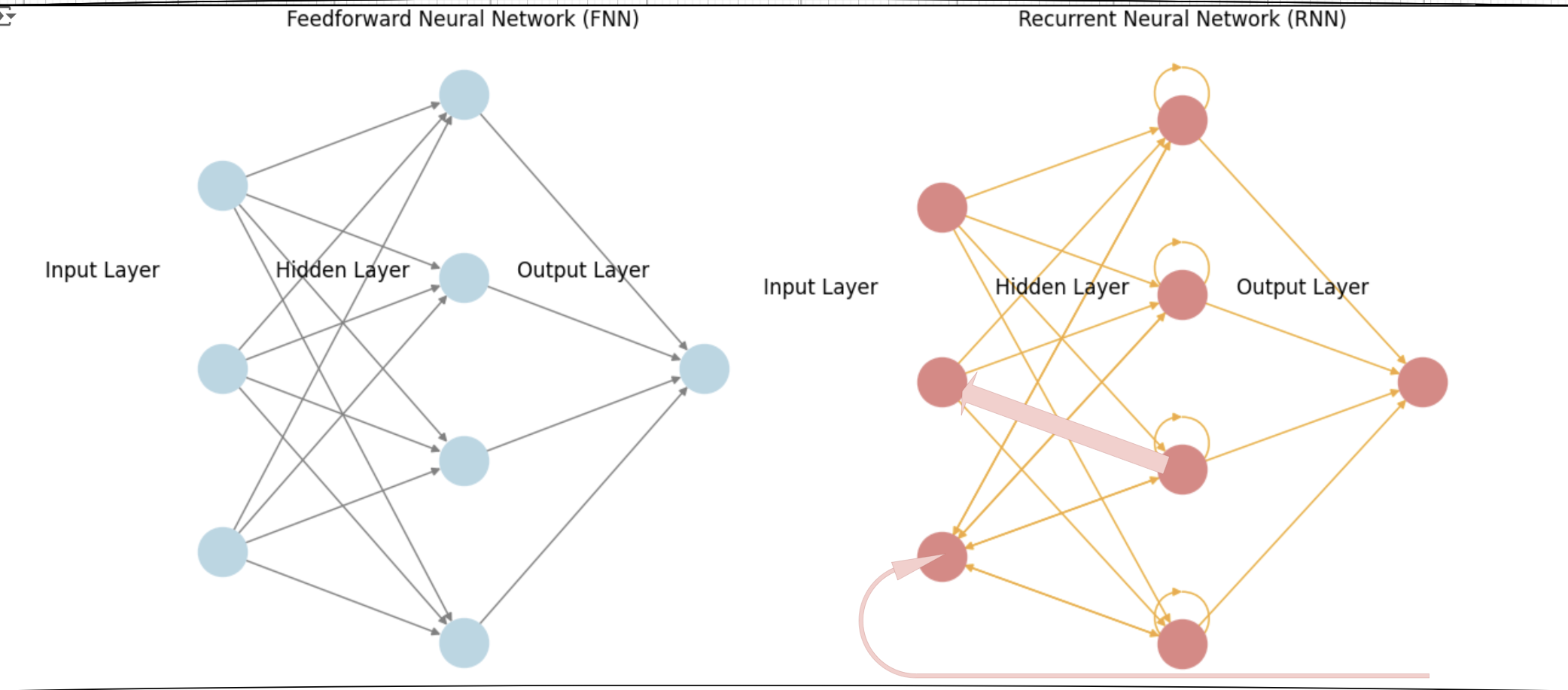
In this article we try to show an example of FNN and for RNN TO understand the math behind it better by comparing to each other: Neural Networks Example Example Setup Input for FNN: Target Output for FNN: RNNs are tailored for sequential data because they are designed to remember and utilize information from previous inputs in a sequence, allowing them to capture temporal relationships and context effectively. This characteristic differentiates RNNs from other neural network types that are not inherently sequence-aware., Input for RNN (Sequence): Target Output for RNN (Sequence): Learning Rate: 1. Feedforward Neural Network (FNN) Structure Input Layer: 1 neuron Hidden Layer: 1 neuron Output Layer: 1 neuron Weights and Biases Initial Weights: (Input to Hidden weight) (Hidden to Output weight) Biases: (Hidden layer bias) (Output layer bias) Step-by-Step Calculation for FNN Step 1: Forward Pass Hidden Layer Output: Output: Step 2: Loss Calculation Using Mean Squared Error (MSE): Step 3: Backward Pass Gradient of Loss with respect to Output: Gradient of Output with respect to Hidden Layer: Gradient of Hidden Layer Output with respect to Weights: Assuming : Step 4: Weight Update Update Output Weight: Update Input Weight: 2. Recurrent Neural Network (RNN) Structure Input Layer: 1 neuron Hidden Layer: 1 neuron Output Layer: 1 neuron Weights and Biases Initial Weights: (Input to Hidden weight) (Hidden to Hidden weight) (Hidden to Output weight) Biases: (Hidden layer bias) (Output layer bias) NOW Lets check Step-by-Step example Calculation for RNN Step 1: Forward Pass Assuming initial hidden state . This is where the memory concept starts; the hidden state retains information from previous time steps. For (Input ): Hidden State: Here, is influenced by the previous hidden state (which is 0). This demonstrates how the RNN maintains memory; the hidden state captures the relevant information to influence future computations. Output: For (Input ): Hidden State: In this step, is influenced by both the current input and the previous hidden state . This reflects the memory of the previous input and its influence on the current state. Output: Step 2: Loss Calculation Using Mean Squared Error (MSE) for the sequence: For : For : Total Loss: Step 3: Backward Pass (BPTT) This is where backpropagation through time takes place. The gradients are computed considering how each hidden state affects the output across the entire sequence. Gradient of Loss w.r.t Output: For : For : Gradient of Output w.r.t Hidden: Gradient of Hidden States: For : For : Memory Influence: The hidden state depends on and the current input . Thus, the gradients also account for the memory stored in previous hidden states. Gradient for Weights: For : For : Step 4: Weight Update Update Weights: For : For : Summary Table Feedforward Neural Network (FNN) StepCalculationForward PassLossGradient (Output)Weight Update Recurrent Neural Network (RNN) StepCalculationExplanationForward PassHidden state remembers (initial state). Hidden state remembers , capturing memory.LossTotal loss calculated across the sequence.Gradient (Output)For Gradients computed for each time step output.Weight UpdateWeights updated based on contributions from all previous states. Key Takeaways FNN: Each input is treated independently, and the backpropagation process is straightforward. RNN: The model retains memory of previous states through the hidden state, making the calculations for gradients more complex, especially during backpropagation through time (BPTT). Each hidden state influences subsequent outputs and reflects the model’s ability to remember past inputs. Another concept to understand here is, memorization in RNNs happens through the hidden states. Each hidden state (h_t) carries information from previous inputs: At time step , the hidden state is influenced by the initial hidden state h_0 (which is 0). At time step , the hidden state is influenced by both the current input and the previous hidden state . Our brief example here was to explain the math behind Feedforward Neural Networks (FNNs) and Recurrent Neural Networks (RNNs) in a simple way, by highlighting their mathematical differences you can understand each model better. https://i.imgur.com/ZfUW6zx.png Don’t forget to check our apps! Visit here….
Understanding RNNs: Why Not compare it with FNN to Understand the Math Behind it Better? – DAY 58