Understanding Keras and Its Role in Deep Learning What is Keras? Keras is an open-source software library that provides a Python interface for artificial neural networks. It serves as a high-level API, simplifying the process of building and training deep learning models. Developed by François Chollet, a researcher at Google, Keras was first released in March 2015. It is designed to enable fast experimentation with deep neural networks, which is crucial for research and development in machine learning and artificial intelligence (AI). Who Invented Keras and Why? François Chollet created Keras to democratize deep learning by making it accessible and easy to use. His goal was to provide a tool that allows for rapid experimentation with neural networks, enabling researchers and developers to prototype and test ideas quickly. The vision behind Keras was to lower the barrier to entry in deep learning, making it possible for more people to contribute to the field. What’s Behind Keras? Keras itself is a high-level wrapper for deep learning frameworks. Initially, it supported multiple backends, including TensorFlow, Theano, and Microsoft Cognitive Toolkit (CNTK). With the release of Keras 3, it now seamlessly integrates with TensorFlow, JAX, and PyTorch, allowing users to choose their preferred backend and switch between them as needed. This multi-backend capability enhances Keras’s flexibility and versatility. Is Keras a Library? Yes, Keras is a library. Specifically, it is a high-level deep learning library written in Python. It abstracts the complexities of deep learning frameworks, providing a simple and consistent interface for building and training neural network models. What Happens When We Import or Use Keras? When you import and use Keras, several things happen behind the scenes: Initialization: Keras initializes the backend framework (TensorFlow, JAX, or PyTorch) you are using, setting up the necessary environment and configurations. Model Building: Keras provides high-level abstractions such as models, layers, optimizers, and loss functions. When you define a model in Keras, it translates your high-level code into operations and structures that the backend framework can execute. Graph Construction: For frameworks like TensorFlow, Keras helps in constructing the computation graph, a directed graph where nodes represent operations and edges represent the flow of data. Data Handling: Keras simplifies data preprocessing, augmentation, and loading, providing utilities to handle various data formats and pipelines. Training Loop: Keras manages the entire training loop, including forward and backward passes, gradient computation, and parameter updates. Evaluation and Prediction: Keras provides simple interfaces for evaluating models on test data and making predictions on new data. Algorithms in Keras Keras supports a wide array of deep learning algorithms, including: Multi-Layer Perceptrons (MLPs): Used for basic classification and regression tasks. Convolutional Neural Networks (CNNs): Used for image and video recognition. Recurrent Neural Networks (RNNs): Used for sequence data such as time series and natural language processing. Use in Machine Learning vs. Deep Learning Keras is primarily used for deep learning tasks due to its design and capabilities. However, it can also be applied to certain machine learning tasks that involve neural networks. Traditional machine learning tasks like decision trees, SVMs, and clustering are typically handled by other libraries like Scikit-Learn. Platforms for Using Keras Keras can be used on various platforms, including: TensorFlow: The primary backend for Keras. Google Colab: An online platform providing free access to GPUs for training models. Amazon Web Services (AWS): For scalable cloud computing. Microsoft Azure: Another cloud platform supporting Keras. Using Keras on Apple Silicon (MLX): Yes, Keras can be used on Apple Silicon (MLX) devices. TensorFlow and Keras support the Apple Silicon architecture, leveraging the performance improvements provided by Apple’s hardware. Latest Developments in 2024 In 2025, Keras continues to evolve with several significant updates: nhanced Model Building: The new ModelBuilder API streamlines the creation of complex neural network architectures, enabling developers to construct sophisticated models with minimal code. reference Improved Data Preprocessing: The DataPreprocessor class offers a comprehensive suite of tools for data cleaning, normalization, and augmentation, simplifying the preparation of datasets for training. reference Advanced Training Techniques: The TrainingOptimizer class facilitates experimentation with various optimization algorithms, learning rates, and regularization methods, enhancing model performance and training efficiency. reference Support for Cutting-Edge Projects: Keras now provides specialized classes such as ImageClassifier, NLPProcessor, GANBuilder, and RLAgent, catering to advanced deep learning projects in image classification, natural language processing, generative adversarial networks, and reinforcement learning. refernce Advanced Techniques and Tools: Keras has integrated support for custom layers, advanced callbacks, transfer learning, hyperparameter tuning, data augmentation, model ensembles, advanced optimizers, regularization techniques, and specialized activation and loss functions, empowering developers to build more efficient and accurate models Advantages of Keras Simplicity: Easy to learn and use, facilitating rapid development. Extensibility: Flexible architecture allows for custom modules. Community Support: Large, active community provides extensive resources, tutorials, and pre-trained models. Speed: Enables faster prototyping and experimentation, with streamlined debugging. Alternatives to Keras and Comparison Other popular deep learning libraries include: PyTorch: Developed by Facebook’s AI Research lab. Known for its dynamic computation graph, which is intuitive and flexible. Strong support for GPU acceleration. Popular in academia for research purposes. Caffe: Developed by the Berkeley Vision and Learning Center (BVLC). Known for its speed and efficiency in deploying models. Less flexible and harder to use compared to Keras and PyTorch. MXNet: Backed by Amazon Web Services (AWS). Supports both symbolic and imperative programming. Highly scalable and suitable for cloud-based applications. Comparison: Ease of Use: Keras is the easiest to use, followed by PyTorch and MXNet. Caffe is the most difficult. Flexibility: PyTorch offers the most flexibility due to its dynamic graph construction. Keras and MXNet are also flexible but in different ways. Performance: Caffe is known for its performance but lacks ease of use. PyTorch and Keras (with TensorFlow) offer competitive performance with better usability. Community and Ecosystem: Keras and PyTorch have large, active communities and extensive ecosystems, making them popular choices. Key Notes: Keras simplifies the process of building, training, and evaluating deep learning models by providing an easy-to-use API. It abstracts the complexities of TensorFlow, making deep learning accessible to a wider audience. By providing a simple, modular, and flexible interface, Keras enables rapid experimentation and development. While there are other deep learning libraries available, Keras stands out for its ease of use and integration with TensorFlow, making it an excellent choice for both beginners and experts in deep learning. Now Let’s Dive into Coding : A Code Example to Understand Keras better now: import tensorflow as tf import matplotlib.pyplot as plt import pandas as pd # Load Fashion MNIST dataset fashion_mnist = tf.keras.datasets.fashion_mnist (X_train_full, y_train_full), (X_test, y_test) = fashion_mnist.load_data() # Split data into training, validation, and test sets X_train, y_train = X_train_full[:-5000], y_train_full[:-5000] X_valid, y_valid = X_train_full[-5000:], y_train_full[-5000:] # Scale pixel values to the 0-1 range X_train, X_valid, X_test = X_train / 255.0, X_valid / 255.0, X_test / 255.0 # Class names for Fashion MNIST class_names = [“T-shirt/top”, “Trouser”, “Pullover”, “Dress”, “Coat”, “Sandal”, “Shirt”, “Sneaker”, “Bag”, “Ankle boot”] # Display the first few images and labels plt.figure(figsize=(10,10)) for i in range(25): plt.subplot(5, 5, i + 1) plt.xticks([]) plt.yticks([]) plt.grid(False) plt.imshow(X_train[i], cmap=plt.cm.binary) plt.xlabel(class_names[y_train[i]]) plt.show() # Set random seed for reproducibility tf.random.set_seed(42) # Here we ate : Building the model using Keras : model = tf.keras.Sequential([ tf.keras.layers.Flatten(input_shape=[28, 28]), tf.keras.layers.Dense(300, activation=”relu”), tf.keras.layers.Dense(100, activation=”relu”), tf.keras.layers.Dense(10, activation=”softmax”) ]) # Compile the model model.compile(loss=”sparse_categorical_crossentropy”, optimizer=”sgd”, metrics=[“accuracy”]) # Train the model history = model.fit(X_train, y_train, epochs=30, validation_data=(X_valid, y_valid)) # Evaluate the model on the test set test_loss, test_acc = model.evaluate(X_test, y_test) print(f”Test accuracy: {test_acc:.4f}”) # Plot training and validation accuracy and loss def plot_learning_curves(history): pd.DataFrame(history.history).plot(figsize=(8, 5)) plt.grid(True) plt.gca().set_ylim(0, 1) # set the vertical range to [0-1] plt.show() plot_learning_curves(history) # Make predictions y_pred = model.predict(X_test) # Plot the first 25 test images, their predicted labels, and the true labels. # Color correct predictions in blue and incorrect predictions in red. plt.figure(figsize=(10,10)) for i in range(25): plt.subplot(5, 5, i + 1) plt.xticks([]) plt.yticks([]) plt.grid(False) plt.imshow(X_test[i], cmap=plt.cm.binary) predicted_label = class_names[y_pred[i].argmax()] true_label = class_names[y_test[i]] color = ‘blue’ if predicted_label == true_label else ‘red’ plt.xlabel(f”{predicted_label} ({true_label})”, color=color) plt.show() These images show the results of the code : Detailed Explanation Importing Libraries import tensorflow as tf import matplotlib.pyplot as plt import pandas as pd In this section, we import the necessary libraries: TensorFlow: Used for building and training the neural network. TensorFlow provides a comprehensive ecosystem for developing machine learning models. Matplotlib: A plotting library used for visualizing the data and the model’s performance over time. Pandas: A data manipulation library that helps in managing and analyzing data, especially for plotting the learning curves. Why Keras is Not Imported Separately Keras is included as part of TensorFlow 2.x and later versions. This means we do not need to import Keras separately because it is available under the tf.keras module. This integration simplifies the workflow and ensures better compatibility and performance optimizations provided by TensorFlow. Loading and Preprocessing Data fashion_mnist = tf.keras.datasets.fashion_mnist (X_train_full, y_train_full), (X_test, y_test) = fashion_mnist.load_data() X_train, y_train = X_train_full[:-5000], y_train_full[:-5000] X_valid, y_valid = X_train_full[-5000:], y_train_full[-5000:] X_train, X_valid, X_test = X_train / 255.0, X_valid / 255.0, X_test / 255.0 Here, we load and preprocess the Fashion MNIST dataset: Load Data: The fashion_mnist.load_data() function loads the dataset, which includes 70,000 grayscale images of 28×28 pixels, divided into training and testing sets. Split Data: We further split the training data into training and validation sets. This is crucial for evaluating the model’s performance on unseen data during training. Normalize Data: We scale the pixel values to the range 0-1 by dividing by 255.0. This normalization helps in speeding up the training process and achieving better convergence. Visualizing Data class_names = ["T-shirt/top", "Trouser", "Pullover", "Dress", "Coat", "Sandal", "Shirt", "Sneaker", "Bag", "Ankle boot"] plt.figure(figsize=(10,10)) for i in range(25): plt.subplot(5, 5, i + 1) plt.xticks([]) plt.yticks([]) plt.grid(False) plt.imshow(X_train[i], cmap=plt.cm.binary) plt.xlabel(class_names[y_train[i]]) plt.show() This section visualizes the first 25 images in the training set: Class Names: We define the class names corresponding to the labels in the dataset. This helps in labeling the images. Plotting Images: We use Matplotlib to plot the first 25 images in a 5×5 grid. The plt.imshow() function displays the images, and the labels are added using the class names. Building the Model tf.random.set_seed(42) model = tf.keras.Sequential([ tf.keras.layers.Flatten(input_shape=[28, 28]), tf.keras.layers.Dense(300, activation="relu"), tf.keras.layers.Dense(100, activation="relu"), tf.keras.layers.Dense(10, activation="softmax") ]) In this section, we build the neural network model: Set Random Seed: Setting the random seed ensures reproducibility of results. This makes debugging and comparing results easier. Sequential Model: We use Keras’ Sequential API to build a linear stack of layers. This is the simplest way to create a model in Keras. Flatten Layer: Converts each 28×28 image into a 1D array of 784 elements, which is required for the fully connected dense layers. Dense Layers: Two hidden layers with 300 and 100…


