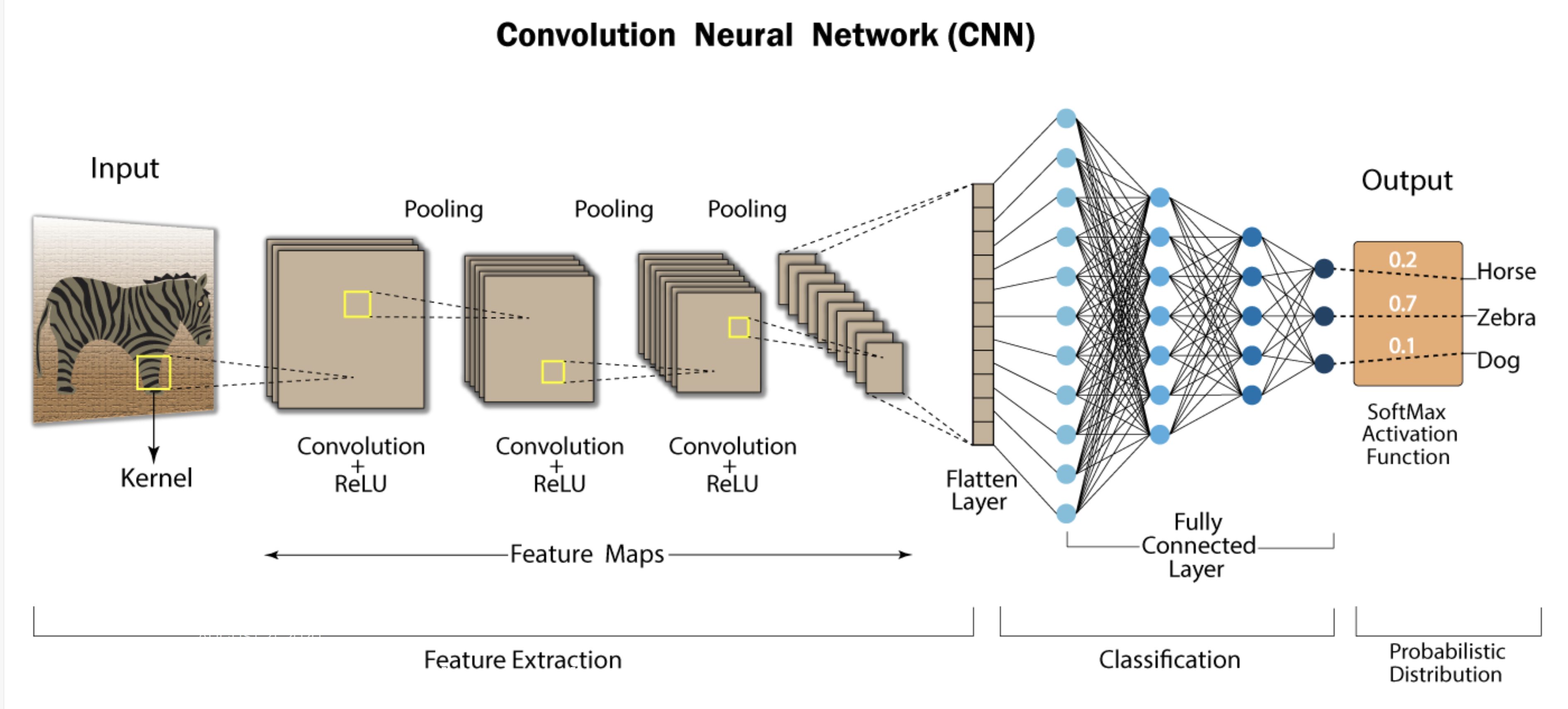
Understanding Convolutional Neural Networks (CNNs): A Step-by-Step Breakdown

Convolutional Neural Networks (CNNs) are widely used in deep learning due to their ability to efficiently process image data. They perform complex operations on input images, enabling tasks like image classification, object detection, and segmentation. This step-by-step guide explains each stage of a CNN’s process, along with an example to clarify the concepts.

1. Input Image Representation

The first step is providing an image to the network as input. Typically, the image is represented as a 3D matrix where the dimensions are:

Height: Number of pixels vertically.
Width: Number of pixels horizontally.
Channels: Number of color channels (e.g., RGB for color images).

Example: A 32×32 RGB image is represented with the shape: (32, 32, 3)

2. Convolutional Layer

The Convolutional Layer applies filters to the image. Filters are small matrices that slide over the image, performing element-wise multiplication followed by summation. This produces feature maps.

Each filter detects specific features like edges or textures. The network learns these filters during training.

Mathematical Operation:
$S(i,j) = \sum_m \sum_n I(i+m, j+n) \cdot K(m,n)$

3. Activation Function (ReLU)

After the convolutional layer, an Activation Function is applied. The most common activation function is ReLU (Rectified Linear Unit), which is mathematically expressed as:

$f(x) = \max(0, x)$

ReLU zeroes out all negative values and retains only positive values, introducing non-linearity into the network.

4. Pooling Layer (Downsampling)

The Pooling Layer reduces the spatial dimensions of the feature maps. This helps reduce the computational complexity of the model and prevents overfitting. The most common pooling operation is Max Pooling.

$P(i,j) = \max(S(i+m, j+n))$

5. Flattening Layer

Before passing data to the fully connected layers, the 2D feature maps are flattened into a 1D vector.

6. Fully Connected Layer

The Fully Connected Layer connects every input neuron to every output neuron, using learned features from earlier layers to make predictions.

7. Output Layer

The final layer in the CNN produces probabilities using a Softmax Activation Function.

$\hat{y}_i = \frac{e^{z_i}}{\sum_j e^{z_j}}$

8. Backpropagation and Optimization

During training, the model uses Backpropagation to calculate the error and update weights. This process ensures the model improves over time by reducing the loss function.

Optimization algorithms: SGD (Stochastic Gradient Descent) or Adam

Step-by-Step Summary of CNN Operations

Step	Operation	Output
1. Input Layer	Receives an image of size (32, 32, 3).	(32, 32, 3)
2. Convolutional Layer	Applies filters to detect features like edges.	(30, 30, 32) (after applying a 3×3 filter)
3. Activation (ReLU)	Applies ReLU to introduce non-linearity.	(30, 30, 32) (negative values set to 0)
4. Pooling Layer	Max pooling reduces the feature map size.	(15, 15, 32)
5. Flattening Layer	Flattens the 2D feature map into a 1D vector.	(7200)
6. Fully Connected Layer	Connects all features to output neurons.	(128)
7. Output Layer	Softmax outputs probabilities for each class.	[0.9, 0.1] (e.g., 90% cat, 10% dog)
8. Backpropagation	Updates weights to minimize error.	Weights updated across layers

Conclusion

This breakdown explains how CNNs process images step-by-step, from input to classification. Each layer plays a specific role in extracting features, learning complex patterns, and improving through backpropagation. CNNs are widely used because of their ability to automatically learn important features and apply them efficiently.

source : https://developersbreach.com/convolution-neural-network-deep-learning/

Step-by-Step Comparison of CNN Operations and Image (Image on Top of Our Article)

In the image on top of our article, we can visualize the entire flow of a typical CNN architecture, which aligns well with the step-by-step table we previously discussed. Here’s how the steps from the table compare to the components shown in the image:

Step	Operation (Table)	Corresponding Component (Image)
1. Input Layer	Receives the image as input, such as a $32 \times 32$ RGB image.	The Input section in the image, showing the zebra image as input.
2. Convolutional Layer	Applies filters (kernels) to detect features like edges.	The first Convolution + ReLU section in the image, where filters are applied to the input image.
3. Activation (ReLU)	Applies ReLU to introduce non-linearity and eliminate negative values.	Part of the Convolution + ReLU layers, shown after the convolution step in the image.
4. Pooling Layer	Applies max pooling to downsample the feature maps and reduce the size of the data.	The Pooling layers in the image, reducing the size of the feature maps.
5. Flattening Layer	Flattens the 2D feature maps into a 1D vector to prepare for the fully connected layer.	The Flatten Layer in the image, located between feature extraction and classification.
6. Fully Connected Layer	Combines all the features and connects them to the output neurons, learning complex representations.	The Fully Connected Layer in the image, where the flattened feature maps are used for classification.
7. Output Layer	Uses the Softmax function to convert logits to probabilities for classification.	The Softmax Activation Function and the Output Layer in the image, showing final class probabilities (e.g., 0.7 for zebra).
8. Backpropagation	Updates the weights based on the loss function during training.	Not explicitly shown in the image, but occurs during training after generating output.

Detailed Comparison: Image Breakdown and Table Alignment

Let’s compare the steps more thoroughly:

Input Layer: The zebra serves as the input in the image, which corresponds to the first step in the table. Here, the image is processed with dimensions like $32 \times 32 \times 3$ .
Convolutional + ReLU Layers: The convolution layers in the image apply filters to detect simple features like edges. These layers are clearly labeled Convolution + ReLU, aligning with the convolution and activation steps in the table.
Pooling Layers: The pooling layers in the image are responsible for downsampling the feature maps. This is a critical step in reducing the spatial dimensions, matching the pooling step in the table.
Flatten Layer: The feature maps are flattened into a 1D vector, as shown in the image. This step prepares the data for classification in the fully connected layers.
Fully Connected Layer: In the image, the fully connected layer learns from the extracted features and combines them for final decision-making. This corresponds to the step in the table where the network connects all features to the output neurons.
Output Layer: The softmax activation function produces probabilistic outputs (e.g., zebra = 0.7). This matches the table’s output layer step, where softmax is applied to determine the class probabilities.
Backpropagation: Although not shown in the image, backpropagation occurs after the output is generated, updating the network’s weights based on the error. This step is essential during training and is listed in the table as well.

Comparing CNN Implementations in PyTorch and MLX

Part 2: Implementing and Comparing CNNs in PyTorch and MLX

We are solving the image classification problem using the ResNet CNN architecture. The CNN will be trained on the CIFAR-10 dataset to classify images into 10 categories (e.g., cats, dogs, airplanes). The aim is to compare the implementation of ResNet in MLX (optimized for Apple Silicon) and PyTorch, a popular deep learning framework. Each framework’s CNN structure will follow the steps discussed in Part 1.

1. MLX CNN Implementation (with CNN steps inside code comments)

MLX Code (ResNet on CIFAR-10)

import mlx.core as mx
import mlx.nn as nn
import mlx.optimizers as optim
import resnet
from dataset import get_cifar10

# Step 1: Define the ResNet-based CNN
# Purpose: ResNet architecture helps solve deep learning problems by using residual connections that reduce vanishing gradient issues.
class ResNetCNN(nn.Module):
    def __init__(self, arch='resnet20'):
        super(ResNetCNN, self).__init__()
        # Step 2: Convolutional Layers (defined inside the ResNet model)
        # ResNet is a CNN with several convolutional layers used to extract features from images
        self.model = getattr(resnet, arch)()

    # Step 3: Forward pass (input -> convolution -> pooling -> fully connected -> output)
    # Purpose: Process images through the CNN layers to make predictions
    def forward(self, x):
        return self.model(x)

# Step 4: Load the CIFAR-10 dataset
# Purpose: CIFAR-10 is a dataset of 10 image classes; used to train and evaluate the CNN
train_data, test_data = get_cifar10(batch_size=256)

# Step 5: Initialize the model, loss function, and optimizer
# Purpose: Cross-entropy loss is used to measure the difference between predicted and actual classes, while Adam optimizer updates weights to minimize this loss
model = ResNetCNN(arch="resnet20")
criterion = nn.CrossEntropyLoss()
optimizer = optim.Adam(model.parameters(), lr=1e-3)

# Step 6: Training loop
# Purpose: Iteratively train the model by adjusting weights over multiple epochs to improve accuracy
for epoch in range(30):
    for batch in train_data:
        inputs, labels = mx.array(batch["image"]), mx.array(batch["label"])
        optimizer.zero_grad()
        outputs = model(inputs)  # Forward pass: Step 3 (input -> output)
        loss = criterion(outputs, labels)  # Compute the loss (prediction vs actual)
        loss.backward()  # Backpropagation to compute gradients
        optimizer.step()  # Update model weights

print("Training complete for MLX ResNet")

2. PyTorch CNN Implementation (with CNN steps inside code comments)

PyTorch Code (ResNet on CIFAR-10)

import torch
import torch.nn as nn
import torch.optim as optim
import torchvision
import torchvision.transforms as transforms

# Step 1: Define the Basic Block (Residual Block) used in ResNet
# Purpose: Each block helps build deeper networks by using residual connections (skip connections) to pass information forward, reducing vanishing gradient problems.
class BasicBlock(nn.Module):
    def __init__(self, in_channels, out_channels, stride=1):
        super(BasicBlock, self).__init__()
        self.conv1 = nn.Conv2d(in_channels, out_channels, kernel_size=3, stride=stride, padding=1)
        self.bn1 = nn.BatchNorm2d(out_channels)
        self.conv2 = nn.Conv2d(out_channels, out_channels, kernel_size=3, padding=1)
        self.bn2 = nn.BatchNorm2d(out_channels)
        self.shortcut = nn.Sequential()  # Skip connection
        if stride != 1 or in_channels != out_channels:
            self.shortcut = nn.Sequential(
                nn.Conv2d(in_channels, out_channels, kernel_size=1, stride=stride),
                nn.BatchNorm2d(out_channels)
            )

    # Step 2: Forward pass for the block (convolution + batch normalization + ReLU)
    # Purpose: Perform the residual connection for each block
    def forward(self, x):
        out = torch.relu(self.bn1(self.conv1(x)))
        out = self.bn2(self.conv2(out))
        out += self.shortcut(x)  # Add the input to the output to form the skip connection
        out = torch.relu(out)
        return out

# Step 3: Define the ResNet model
# Purpose: ResNet model consisting of multiple blocks, used for image classification
class ResNetCNN(nn.Module):
    def __init__(self, block, num_blocks, num_classes=10):
        super(ResNetCNN, self).__init__()
        self.in_channels = 64
        self.conv1 = nn.Conv2d(3, 64, kernel_size=3, stride=1, padding=1)  # Initial convolution
        self.bn1 = nn.BatchNorm2d(64)
        self.layer1 = self._make_layer(block, 64, num_blocks[0], stride=1)
        self.layer2 = self._make_layer(block, 128, num_blocks[1], stride=2)
        self.layer3 = self._make_layer(block, 256, num_blocks[2], stride=2)
        self.layer4 = self._make_layer(block, 512, num_blocks[3], stride=2)
        self.linear = nn.Linear(512, num_classes)  # Fully connected layer for final classification

    # Step 4: Define layer construction method
    # Purpose: Create the sequential layers of blocks in ResNet
    def _make_layer(self, block, out_channels, num_blocks, stride):
        strides = [stride] + [1] * (num_blocks - 1)
        layers = []
        for stride in strides:
            layers.append(block(self.in_channels, out_channels, stride))
            self.in_channels = out_channels
        return nn.Sequential(*layers)

    # Step 5: Forward pass through the ResNet model (input -> conv -> pooling -> fully connected -> output)
    def forward(self, x):
        out = torch.relu(self.bn1(self.conv1(x)))
        out = self.layer1(out)
        out = self.layer2(out)
        out = self.layer3(out)
        out = self.layer4(out)
        out = torch.flatten(out, 1)
        out = self.linear(out)  # Fully connected layer
        return out

# Step 6: Load CIFAR-10 dataset
# Purpose: Load and preprocess the image data
transform = transforms.Compose([transforms.ToTensor(), transforms.Normalize((0.5, 0.5, 0.5), (0.5, 0.5, 0.5))])
trainset = torchvision.datasets.CIFAR10(root='./data', train=True, download=True, transform=transform)
trainloader = torch.utils.data.DataLoader(trainset, batch_size=256, shuffle=True)

# Step 7: Initialize the model, loss function, and optimizer
# Purpose: Cross-entropy loss is used to measure the classification error, and the Adam optimizer adjusts the weights to reduce this error
device = torch.device('mps' if torch.backends.mps.is_available() else 'cpu')
model = ResNetCNN(BasicBlock, [2, 2, 2, 2]).to(device)
criterion = nn.CrossEntropyLoss()
optimizer = optim.Adam(model.parameters(), lr=0.001)

# Step 8: Training loop
# Purpose: Iterate over the dataset to train the model and optimize weights
for epoch in range(30):
    running_loss = 0.0
    for i, data in enumerate(trainloader, 0):
        inputs, labels = data
        inputs, labels = inputs.to(device), labels.to(device)
        
        optimizer.zero_grad()
        outputs = model(inputs)  # Forward pass: CNN steps (input -> conv -> pooling -> fully connected -> output)
        loss = criterion(outputs, labels)  # Compute the loss (prediction vs actual)
        loss.backward()  # Backpropagation to compute gradients
        optimizer.step()  # Update model weights

        running_loss += loss.item()
        if i % 100 == 99:
            print(f'[Epoch {epoch + 1}, Batch {i + 1}] loss: {running_loss / 100:.3f}')
            running_loss = 0.0

print('Finished Training for PyTorch ResNet')

3. Comparison of MLX and PyTorch Implementations

MLX Code: The MLX code is shorter and more abstract because MLX provides a high-level API that includes pre-built architectures like ResNet. This simplifies the process for the user, and the framework is optimized for Apple Silicon, meaning it can take advantage of the M1/M2 chips for better performance.
PyTorch Code: In contrast, PyTorch requires you to manually define each layer and block of the architecture, which results in more flexibility but also much longer code. While PyTorch supports GPU acceleration through MPS (Metal Performance Shaders) on Apple Silicon, it does not take full advantage of the hardware’s deep optimization like MLX does.

Key Differences:

Abstraction vs. Control: MLX simplifies the process by abstracting most of the architecture, allowing you to focus on training. PyTorch, however, gives you full control to design and tweak each part of the model.
Performance: MLX is better optimized for Apple hardware, particularly for leveraging the Neural Engine. PyTorch works with MPS, but its deep learning optimizations are more generalized.
Development Time: MLX allows for quicker implementation and reduced development time due to pre-built models, while PyTorch requires more manual effort but provides flexibility and customization.

Conclusion:

Both frameworks are useful depending on the user’s goals. MLX is best for those looking for high performance on Apple hardware and faster development cycles. On the other hand, PyTorch offers greater flexibility and is better suited for research and custom model development, albeit at the cost of more complex and longer code.

CNN- Convolutional Neural Networks – DAY 53