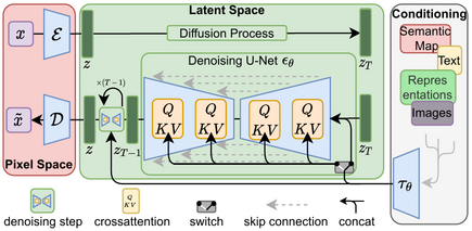
Unveiling Diffusion Models: From Denoising to Generative Art

The field of generative modeling has witnessed remarkable advancements over the past few years, with diffusion models emerging as a powerful class capable of generating high-quality, diverse images and other data types. Rooted in concepts from thermodynamics and stochastic processes, diffusion models have not only matched but, in some aspects, surpassed the performance of traditional generative models like Generative Adversarial Networks (GANs) and Variational Autoencoders (VAEs). In this blog post, we’ll delve deep into the evolution of diffusion models, understand their underlying mechanisms, and explore their wide-ranging applications and future prospects.

---

Table of Contents

1. Introduction to Diffusion Models
2. Historical Development
3. Understanding Diffusion Models
   • The Forward Diffusion Process (Noising)
   • The Reverse Diffusion Process (Denoising)
   • Training Objective
   • Variance Scheduling
4. Model Architecture
5. Implementing Diffusion Models
6. Applications of Diffusion Models
7. Advancements: Latent Diffusion Models and Beyond
8. Challenges and Limitations
9. Future Directions
10. Conclusion
11. References
12. Additional Resources

---

Introduction to Diffusion Models

Diffusion models are a class of probabilistic generative models that learn data distributions by modeling the gradual corruption and subsequent recovery of data through a Markov chain of diffusion steps. The core idea is to learn how to reverse a predefined noising process that progressively adds noise to the data until it becomes indistinguishable from pure noise. By learning this reverse process, the model can generate new data samples starting from random noise.

The Conceptual Foundation

The inspiration for diffusion models comes from non-equilibrium thermodynamics and stochastic differential equations, particularly the concept of Langevin dynamics. In physics, diffusion processes describe the random movement of particles suspended in a medium, resulting from collisions with the medium’s molecules. Similarly, in diffusion models, data points undergo random perturbations, and the model learns to reverse these perturbations to recover the original data distribution.

---

Historical Development

Early Foundations

The theoretical foundations of diffusion models date back to earlier works on score matching and denoising autoencoders. In particular, Score Matching, introduced by Aapo Hyvärinen in 2005^[1], involves estimating the gradient of the log-density (the score function) of a data distribution, which is central to diffusion models.

Formalization of Diffusion Models

In 2015, Jascha Sohl-Dickstein et al. formalized diffusion models in their paper “Deep Unsupervised Learning using Nonequilibrium Thermodynamics”^[2]. They introduced the concept of modeling the data distribution through a diffusion process and learning to reverse it to generate new data. Although their results were promising, diffusion models didn’t receive significant attention at the time due to the rising popularity of GANs.

Breakthrough with DDPM

The turning point came in 2020 when Jonathan Ho, Ajay Jain, and Pieter Abbeel introduced Denoising Diffusion Probabilistic Models (DDPMs)^[3]. They demonstrated that diffusion models could generate high-fidelity images comparable to those produced by GANs. Their approach involved a refined training objective and an emphasis on the connection between diffusion models and variational inference.

Figure 1: Comparison of images generated by GANs and DDPMs

To see a comparison between images generated by GANs and DDPMs, refer to Figure 9 in the DDPM paper: “Denoising Diffusion Probabilistic Models”
Link: https://arxiv.org/abs/2006.11239

Improvements and Advancements

Building upon DDPM, researchers from OpenAI, including Alexander Quinn Nichol and Prafulla Dhariwal, proposed several improvements in their 2021 paper “Improved Denoising Diffusion Probabilistic Models”^[4]. They introduced techniques like:

• Modified Variance Schedules: Adjusting the noise schedule to improve sample quality.
• Training with Larger Models: Demonstrating that scaling up the model size leads to better results.
• Hybrid Objectives: Combining different loss functions to enhance training stability and performance.

Notable Diffusion Model Papers in 2024

GenPercept and StableNormal: These models introduced single-step diffusion to improve efficiency, focusing on enhancing visual texture and reducing interference during image generation tasks. StableNormal’s two-stage refinement strategy led to high precision in visual details, essential for tasks requiring intricate accuracy. Link: https://ar5iv.org/abs/2409.18124

SiT (Scalable Interpolant Transformers): This model combines flow and diffusion techniques to enhance scalability and sample quality, improving high-resolution image synthesis and adding flexibility to diffusion pathways. By dynamically fine-tuning these pathways, SiT achieves better performance in generative applications. Link: https://ar5iv.org/abs/2401.08740

Lotus: The Lotus model applies diffusion principles to dense prediction tasks, such as monocular depth and surface normal estimation, and employs stochastic methods to predict uncertainty in visual tasks. It effectively maintains detail without increasing model complexity, achieving outstanding results in tasks requiring dense, fine-grained predictions. Link: https://ar5iv.org/abs/2405.12399

---

Understanding Diffusion Models

The Forward Diffusion Process (Noising)

The forward process gradually adds noise to the data over \( T \) time steps, transforming an original data sample \( \mathbf{x}_0 \) into a noise vector \( \mathbf{x}_T \). At each time step \( t \), Gaussian noise is added according to:

\( q(\mathbf{x}_t | \mathbf{x}_{t-1}) = \mathcal{N}(\mathbf{x}_t; \sqrt{1 – \beta_t} \mathbf{x}_{t-1}, \beta_t \mathbf{I}) \)

• \( \beta_t \) is a small positive variance term that controls the amount of noise added at each step.
• \( \mathbf{I} \) is the identity matrix, ensuring isotropic noise.

Table 1: Summary of Notations

Symbol	Description
\( \mathbf{x}_0 \)	Original data sample
\( \mathbf{x}_t \)	Noisy data at time step \( t \)
\( \beta_t \)	Variance schedule controlling noise addition
\( \alpha_t \)	Defined as \( 1 – \beta_t \)
\( \bar{\alpha}_t \)	Cumulative product \( \prod_{s=1}^{t} \alpha_s \)

An important property is that we can sample \( \mathbf{x}_t \) at any time step directly from \( \mathbf{x}_0 \) using the closed-form solution:

\( q(\mathbf{x}_t | \mathbf{x}_0) = \mathcal{N}(\mathbf{x}_t; \sqrt{\bar{\alpha}_t} \mathbf{x}_0, (1 – \bar{\alpha}_t) \mathbf{I}) \)

This property allows efficient computation without iterating through all intermediate steps.

Figure 2: Visualization of the Forward Diffusion Process

For a visual explanation of how noise is added over time, see Figure 2 in the blog post “An Introduction to Diffusion Models for Machine Learning” on Lil’Log: Understanding Diffusion Models

The Reverse Diffusion Process (Denoising)

The reverse process aims to recover \( \mathbf{x}_0 \) from \( \mathbf{x}_T \) by iteratively removing noise:

\( p_\theta(\mathbf{x}_{t-1} | \mathbf{x}_t) = \mathcal{N}(\mathbf{x}_{t-1}; \mu_\theta(\mathbf{x}_t, t), \Sigma_\theta(\mathbf{x}_t, t)) \)

Training Objective

The training objective derives from variational inference and can be simplified to a weighted sum of denoising score matching losses at each time step:

\( L = \mathbb{E}_{\mathbf{x}_0, \boldsymbol{\epsilon}, t} \left[ \left\| \boldsymbol{\epsilon} – \boldsymbol{\epsilon}_\theta(\mathbf{x}_t, t) \right\|^2 \right] \)

Variance Scheduling

The variance schedule \( \beta_t \) plays a crucial role in the model’s performance. Common choices include linear schedules, but later works have proposed cosine schedules^[4] and learned schedules for better results.

For example, the cosine schedule is defined as:

\( \bar{\alpha}_t = \frac{f(t)}{f(0)} \quad \text{where} \quad f(t) = \cos\left( \frac{t / T + s}{1 + s} \cdot \frac{\pi}{2} \right)^2 \)

The Reverse Sampling Equation

The update equation for one reverse diffusion step is:

\( \mathbf{x}_{t-1} = \frac{1}{\sqrt{\alpha_t}} \left( \mathbf{x}_t – \frac{1 – \alpha_t}{\sqrt{1 – \bar{\alpha}_t}} \boldsymbol{\epsilon}_\theta(\mathbf{x}_t, t) \right) + \sigma_t \mathbf{z} \)

• \( \sigma_t \) is a variance term, often set to \( \sqrt{\beta_t} \).
• \( \mathbf{z} \) is standard Gaussian noise.

---

Model Architecture

U-Net Backbone

The most successful diffusion models utilize a U-Net architecture^[5] as the backbone for \( \boldsymbol{\epsilon}_\theta(\mathbf{x}_t, t) \). The U-Net is an encoder-decoder network with skip connections, allowing it to capture both global and local features efficiently.

• Downsampling Path: Extracts features at multiple scales.
• Upsampling Path: Reconstructs the image while integrating features from the downsampling path via skip connections.

Figure 5: U-Net Architecture

To see an illustration of the U-Net architecture, refer to Figure 1 in the original U-Net paper: “U-Net: Convolutional Networks for Biomedical Image Segmentation”
Link: https://arxiv.org/abs/1505.04597

Incorporating Time Steps

• Positional Encoding: Similar to Transformers, the scalar time \( t \) is transformed into a higher-dimensional vector using sinusoidal functions.
• Learned Embeddings: Alternatively, \( t \) can be embedded using learned embeddings passed through embedding layers.

Attention Mechanisms

Some diffusion models incorporate attention mechanisms, such as multi-head self-attention, to capture long-range dependencies in the data. This is particularly beneficial for high-resolution images where global coherence is important.

---

Implementing Diffusion Models

1. Data Preparation:
   • Normalize data to have zero mean and unit variance.
   • Compute the variance schedule \( \beta_t \) and cumulative products \( \bar{\alpha}_t \).
2. Model Definition:
   • Use a U-Net architecture with appropriate modifications.
   • Incorporate time embeddings.
3. Training Loop:
   • For each batch:
     • Sample random \( t \) and noise \( \boldsymbol{\epsilon} \).
     • Generate \( \mathbf{x}_t \) using the forward process.
     • Compute the loss between \( \boldsymbol{\epsilon} \) and \( \boldsymbol{\epsilon}_\theta(\mathbf{x}_t, t) \).
   • Optimize the model parameters using the chosen optimizer.
4. Sampling (Generation):
   • Start from \( \mathbf{x}_T \sim \mathcal{N}(\mathbf{0}, \mathbf{I}) \).
   • Iteratively apply the reverse process to obtain \( \mathbf{x}_{t-1} \) from \( \mathbf{x}_t \).
   • After \( T \) steps, obtain \( \mathbf{x}_0 \), a generated data sample.

Algorithm 1: Pseudocode for Training and Sampling

# Training
for each epoch:
    for each batch of data x0:
        t ~ Uniform(1, T)
        ε ~ N(0, I)
        xt = sqrt(ᾱ_t) * x0 + sqrt(1 - ᾱ_t) * ε
        Loss = ||ε - εθ(xt, t)||^2
        Backpropagate and update θ

# Sampling
xT ~ N(0, I)
for t from T to 1:
    z ~ N(0, I) if t > 1 else 0
    x_{t-1} = (1 / sqrt(α_t)) * (xt - (1 - α_t) / sqrt(1 - ᾱ_t) * εθ(xt, t)) + σ_t * z
    xt = x_{t-1}
  

For a detailed implementation guide, you can refer to the blog post by Hugging Face: “Diffusion Models: A Practical Guide”
Link: https://huggingface.co/blog/annotated-diffusion

---

Applications of Diffusion Models

Image Generation

Diffusion models have been successful in generating high-resolution, high-fidelity images across various datasets, including:

• ImageNet: Generating diverse images conditioned on class labels.
• Face Generation: Producing realistic human faces.

Figure 6: Images Generated by Diffusion Models

You can view samples of images generated by diffusion models in the official OpenAI blog post: “Cascaded Diffusion Models for High-Resolution Image Synthesis”
Link: https://openai.com/blog/diffusion-models/

Text-to-Image Synthesis

By conditioning the diffusion process on text embeddings (e.g., from a language model), diffusion models can generate images from textual descriptions. This has led to models like:

• DALL·E 2: Developed by OpenAI, combining CLIP embeddings with diffusion models^[6].
• Imagen: From Google Research, utilizing large language models for text conditioning^[7].

Figure 7: Text-to-Image Generation Examples

Explore examples of text-to-image synthesis on the OpenAI DALL·E 2 page: “DALL·E 2 Examples”
Link: https://openai.com/dall-e-2/

Audio and Speech Generation

Diffusion models have been adapted for audio synthesis, including:

• WaveGrad: For generating raw audio waveforms^[8].
• DiffWave: For text-to-speech applications^[9].

Figure 8: Audio Waveform Generation

Listen to audio samples generated by WaveGrad on their GitHub repository: “WaveGrad Audio Samples”
Link: https://github.com/lmnt-com/wavegrad

Molecular Generation

In computational chemistry and drug discovery, diffusion models can generate novel molecular structures with desired properties^[10].

Figure 9: Molecules Generated by Diffusion Models

For examples of molecule generation, refer to the paper “Score-Based Generative Modeling in Latent Space” and its associated GitHub repository: “Molecule Generation Examples”
Link: https://github.com/yang-song/score_flow

Super-Resolution and Inpainting

Diffusion models can enhance image resolution and fill in missing or corrupted parts of images, leveraging their strong generative capabilities.

Figure 10: Image Super-Resolution with Diffusion Models

See examples of super-resolution in the paper “Enhanced Super-Resolution through Attention to Texture and Structure”
Link: https://arxiv.org/abs/2102.01691

---

Advancements: Latent Diffusion Models and Beyond

Latent Diffusion Models (LDMs)

To address the computational challenges of operating in high-dimensional data spaces, Latent Diffusion Models^[11] perform diffusion in a lower-dimensional latent space learned by an autoencoder.

• Autoencoder Framework:
  • Encoder: Compresses data into latent representations.
  • Decoder: Reconstructs data from latent space.
• Diffusion in Latent Space: Reduces computational load and accelerates sampling.

Figure 11: Latent Diffusion Model Framework

For an in-depth explanation and visualizations, refer to the Latent Diffusion Models paper: “High-Resolution Image Synthesis with Latent Diffusion Models”
Link: https://arxiv.org/abs/2112.10752

Stable Diffusion

Stable Diffusion^[12] is a prominent example of an LDM that has been open-sourced, providing powerful text-to-image generation capabilities. It leverages:

• Efficient Training: By operating in latent space, training becomes more feasible on limited hardware.
• Flexible Conditioning: Supports conditioning on text prompts, images, and other modalities.

Figure 12: Images Generated by Stable Diffusion

Explore a gallery of images generated by Stable Diffusion on their official website: “Stable Diffusion Showcase”
Link: https://stability.ai/stablediffusion

Accelerating Sampling

A major focus has been reducing the number of diffusion steps required for generation, leading to faster sampling times. Techniques include:

• Denoising Diffusion Implicit Models (DDIM): Deterministic sampling methods that require fewer steps^[13].
• Knowledge Distillation: Training smaller models to mimic larger ones in fewer steps.

---

Challenges and Limitations

While diffusion models have shown great promise, they come with challenges:

• Computational Cost: Training and sampling can be resource-intensive, especially for high-resolution data.
• Model Complexity: The need for large models and careful tuning of hyperparameters.
• Sampling Speed: Even with improvements, generating samples can be slower compared to GANs.
• Interpretability: Understanding the internal workings and decision-making process is non-trivial.

---

Future Directions

The research community is actively exploring ways to:

• Enhance Efficiency: Developing algorithms for faster sampling and more efficient training.
• Extend Modalities: Applying diffusion models to other data types like video, 3D models, and more.
• Improve Control: Allowing finer control over generated outputs through better conditioning methods.
• Integrate with Other Models: Combining diffusion models with other architectures like Transformers for synergistic effects.
• Theoretical Understanding: Deepening the theoretical foundations to better understand why diffusion models perform so well.

Practical Example for Diffusion Model: Understanding Through Code

This example is ideal for anyone aiming to grasp the core concepts of diffusion models through practical application, as it guides you from setting up the variance schedule to generating images with the reverse diffusion process.

1. Variance Schedule: Controlling the Diffusion Process

The diffusion process gradually adds noise to an image until it is unrecognizable. By controlling the rate of noise addition, we can ensure a smooth transition. The function variance_schedule defines the schedule parameters α, α_cumprod, and β for each step.

import numpy as np

def variance_schedule(T, s=0.008, max_beta=0.999):
    t = np.arange(T + 1)
    f = np.cos((t / T + s) / (1 + s) * np.pi / 2) ** 2
    alpha = np.clip(f[1:] / f[:-1], 1 - max_beta, 1)
    alpha = np.append(1, alpha).astype(np.float32)  # add α₀ = 1
    beta = 1 - alpha
    alpha_cumprod = np.cumprod(alpha)
    return alpha, alpha_cumprod, beta  # αₜ , α̅ₜ , βₜ for t = 0 to T

T = 4000
alpha, alpha_cumprod, beta = variance_schedule(T)

Explanation:

• T: Total number of diffusion steps, controlling the depth of the noise addition.
• s: A tiny constant to prevent instability at the start.
• max_beta: Prevents the variance (β) from becoming too large, which could destabilize the model.
• alpha, beta, alpha_cumprod: alpha is the scaling factor, beta controls added noise at each step, and alpha_cumprod is the cumulative product of alpha values across time steps, ensuring a gradual transition from a clean to a fully noisy image.

2. Preparing Batches for Training

The prepare_batch function prepares the images with added noise at various time steps, which are used to train the model.

import tensorflow as tf

def prepare_batch(X):
    # Scale from [-1, +1]
    X = tf.cast(X[..., tf.newaxis], tf.float32) * 2 - 1
    X_shape = tf.shape(X)
    t = tf.random.uniform([X_shape[0]], minval=1, maxval=T + 1, dtype=tf.int32)
    alpha_cm = tf.gather(alpha_cumprod, t)
    alpha_cm = tf.reshape(alpha_cm, [X_shape[0]] + [1] * (len(X_shape) - 1))
    noise = tf.random.normal(X_shape)
    return {
        "X_noisy": alpha_cm ** 0.5 * X + (1 - alpha_cm) ** 0.5 * noise,
        "time": t,
    }, noise

Explanation:

• Scaling: Scales pixel values to the range [-1, 1], matching the Gaussian noise format.
• Random Time Step Selection: Selects a random time step for each image to simulate different noise levels.
• Noise Addition: Applies Gaussian noise to each image based on the current time step, using cumulative scaling factors.

3. Dataset Preparation

The prepare_dataset function organizes images into batches for training and validation, applying the prepare_batch function.

def prepare_dataset(X, batch_size=32, shuffle=False):
    ds = tf.data.Dataset.from_tensor_slices(X)
    if shuffle:
        ds = ds.shuffle(buffer_size=10_000)
    return ds.batch(batch_size).map(prepare_batch).prefetch(1)

# Example usage:
train_set = prepare_dataset(X_train, batch_size=32, shuffle=True)
valid_set = prepare_dataset(X_valid, batch_size=32)

Explanation:

• Batching and Shuffling: The function batches images, shuffling the training dataset to improve model generalization.
• Mapping: The prepare_batch function is applied to each batch to prepare noisy images with their time steps.

4. Building the Diffusion Model

The diffusion model architecture is defined here, using a U-Net structure to learn noise removal at each time step.

def build_diffusion_model():
    X_noisy = tf.keras.layers.Input(shape=[28, 28, 1], name="X_noisy")
    time_input = tf.keras.layers.Input(shape=[], dtype=tf.int32, name="time")
    # [...] Build the model layers based on the noisy images and the time steps
    outputs = [...]  # Predict the noise (output shape should match input images)
    return tf.keras.Model(inputs=[X_noisy, time_input], outputs=[outputs])

Explanation:

• Inputs: X_noisy (noisy images) and time_input (time steps).
• Architecture: Uses a U-Net structure with convolutional layers and skip connections to handle noise removal based on noisy images and their corresponding time steps.

5. Training the Model

The model is trained with Huber loss and the Nadam optimizer, which are suitable choices for this type of problem.

model = build_diffusion_model()
model.compile(loss=tf.keras.losses.Huber(), optimizer="nadam")
history = model.fit(train_set, validation_data=valid_set, epochs=100)

Explanation:

• Loss Function: Huber loss provides a balance between sensitivity to outliers and stability in optimization, useful for learning subtle noise adjustments.
• Training: Runs for 100 epochs, comparing performance on validation data to avoid overfitting.

6. Image Generation with Reverse Diffusion Process

This function generates images by reversing the noise addition process, starting from a Gaussian noise image.

def generate(model, batch_size=32):
    X = tf.random.normal([batch_size, 28, 28, 1])
    for t in range(T, 0, -1):
        noise = tf.random.normal(tf.shape(X)) if t > 1 else tf.zeros(tf.shape(X))
        X_noise = model({
            "X_noisy": X,
            "time": tf.constant([t] * batch_size)
        })
        X = (
            1 / (alpha[t] ** 0.5) *
            (X - beta[t] / ((1 - alpha_cumprod[t]) ** 0.5) * X_noise) +
            (1 - alpha[t]) ** 0.5 * noise
        )
    return X

X_gen = generate(model)  # generated images

Explanation:

• Noise Initialization: Starts with random Gaussian noise, simulating an image obscured by noise.
• Reverse Process: Iteratively removes noise using predicted noise from the model, gradually reconstructing an image by applying the reverse diffusion process.
• Image Output: Returns generated images resembling the original dataset after the reverse diffusion completes.

Conclusion

This example walks you through each step of implementing a diffusion model, from setting up the variance schedule to the generation of images. By using a diffusion model, we’re able to produce high-quality, diverse images by learning the gradual process of adding and removing noise. The code here provides a thorough understanding of each step, making it a great way to learn how diffusion models operate and gain hands-on experience in building one from scratch. also the theoretical part made you understand how diffusion was invented from first place and how it works. Check the references and links to understand more

References

[1]: Hyvärinen, A. (2005). Estimation of Non-Normalized Statistical Models by Score Matching. Journal of Machine Learning Research, 6, 695–709.

[2]: Sohl-Dickstein, J., Weiss, E., Maheswaranathan, N., & Ganguli, S. (2015). Deep Unsupervised Learning using Nonequilibrium Thermodynamics. Proceedings of the 32nd International Conference on Machine Learning, 2256–2265.
Link: https://arxiv.org/abs/1503.03585

[3]: Ho, J., Jain, A., & Abbeel, P. (2020). Denoising Diffusion Probabilistic Models. Advances in Neural Information Processing Systems, 33, 6840–6851.
Link: https://arxiv.org/abs/2006.11239

[4]: Nichol, A. Q., & Dhariwal, P. (2021). Improved Denoising Diffusion Probabilistic Models. Proceedings of the 38th International Conference on Machine Learning, 8162–8171.
Link: https://arxiv.org/abs/2102.09672

[5]: Ronneberger, O., Fischer, P., & Brox, T. (2015). U-Net: Convolutional Networks for Biomedical Image Segmentation. Medical Image Computing and Computer-Assisted Intervention, 234–241.
Link: https://arxiv.org/abs/1505.04597

[6]: Ramesh, A., et al. (2022). Hierarchical Text-Conditional Image Generation with CLIP Latents. arXiv preprint arXiv:2204.06125.
Link: https://arxiv.org/abs/2204.06125

[7]: Saharia, C., et al. (2022). Photorealistic Text-to-Image Diffusion Models with Deep Language Understanding. arXiv preprint arXiv:2205.11487.
Link: https://arxiv.org/abs/2205.11487

[8]: Chen, N., Zhang, Y., Zen, H., Weiss, R. J., Norouzi, M., & Chan, W. (2020). WaveGrad: Estimating Gradients for Waveform Generation. arXiv preprint arXiv:2009.00713.
Link: https://arxiv.org/abs/2009.00713

[9]: Kong, Z., Ping, W., Huang, J., Zhao, K., & Catanzaro, B. (2020). DiffWave: A Versatile Diffusion Model for Audio Synthesis. arXiv preprint arXiv:2009.09761.
Link: https://arxiv.org/abs/2009.09761

[10]: Hoogeboom, E., et al. (2022). Equivariant Diffusion for Molecule Generation in 3D. arXiv preprint arXiv:2203.17003.
Link: https://arxiv.org/abs/2203.17003

[11]: Rombach, R., Blattmann, A., Lorenz, D., Esser, P., & Ommer, B. (2022). High-Resolution Image Synthesis with Latent Diffusion Models. Proceedings of the IEEE/CVF Conference on Computer Vision and Pattern Recognition, 10684–10695.
Link: https://arxiv.org/abs/2112.10752

[12]: Stable Diffusion – Stable Diffusion. Retrieved from
Link: https://stability.ai/stablediffusion

[13]: Song, J., Meng, C., & Ermon, S. (2020). Denoising Diffusion Implicit Models. arXiv preprint arXiv:2010.02502.
Link: https://arxiv.org/abs/2010.02502

---

Additional Resources

• KerasCV: The Keras Computer Vision library includes implementations of diffusion models, making it accessible for practitioners to experiment with these models.
  KerasCV GitHub Repository: https://github.com/keras-team/keras-cv
• OpenAI’s GLIDE: A diffusion model for text-guided image synthesis, demonstrating the versatility of the approach.
  GLIDE Paper: “GLIDE: Towards Photorealistic Image Generation and Editing with Text-Guided Diffusion Models”
  Link: https://arxiv.org/abs/2112.10741
• Hugging Face Diffusers: A library that provides pretrained diffusion models and tools for inference and training.
  Hugging Face Diffusers Library: https://github.com/huggingface/diffusers
• Community Projects: Numerous repositories and projects on GitHub provide implementations and extensions of diffusion models, fostering collaborative development.
  Awesome Diffusion Models: https://github.com/heejkoo/Awesome-Diffusion-Models

---

GANs vs Diffusion Models Comparison (2025 Update)