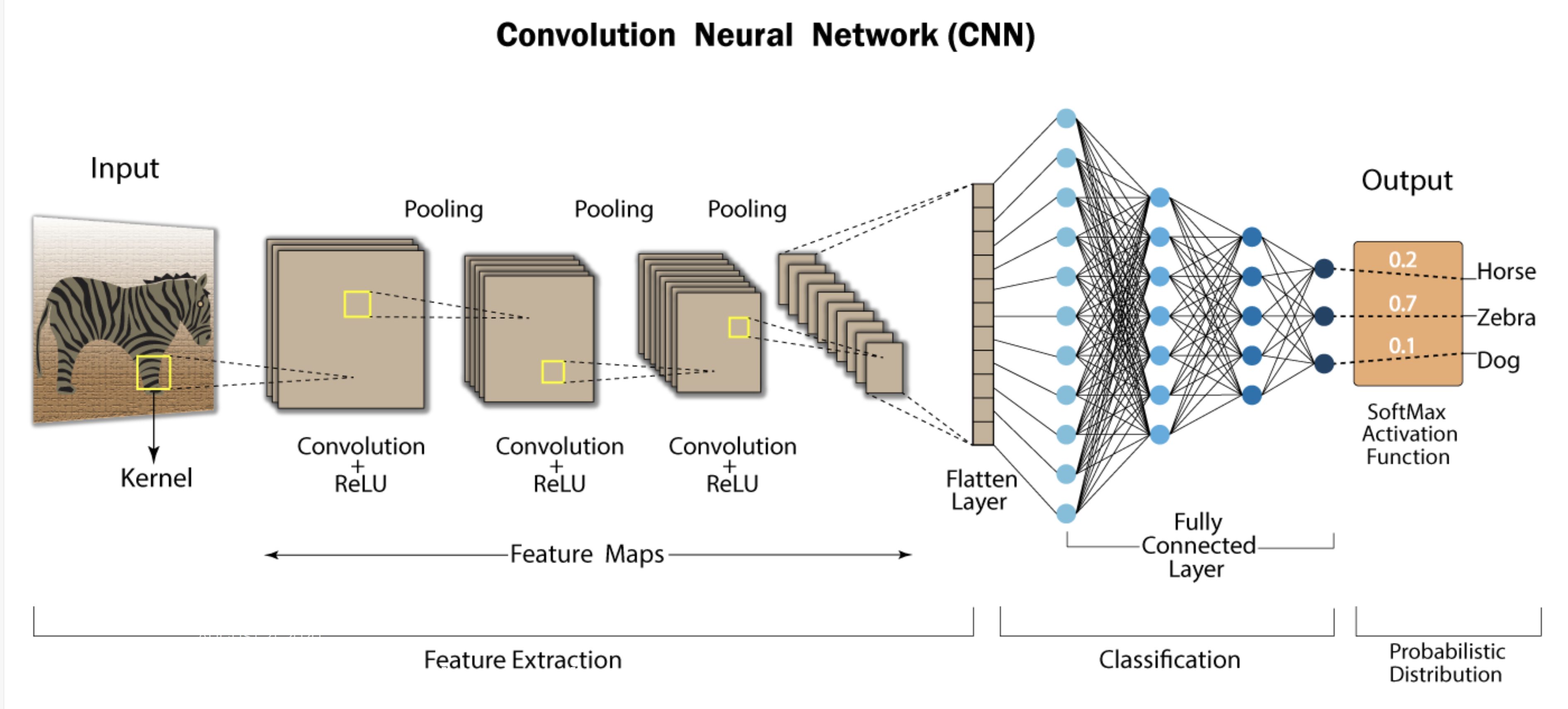
CNN – Convolutional Neural Networks explained by INGOAMPT – DAY 53

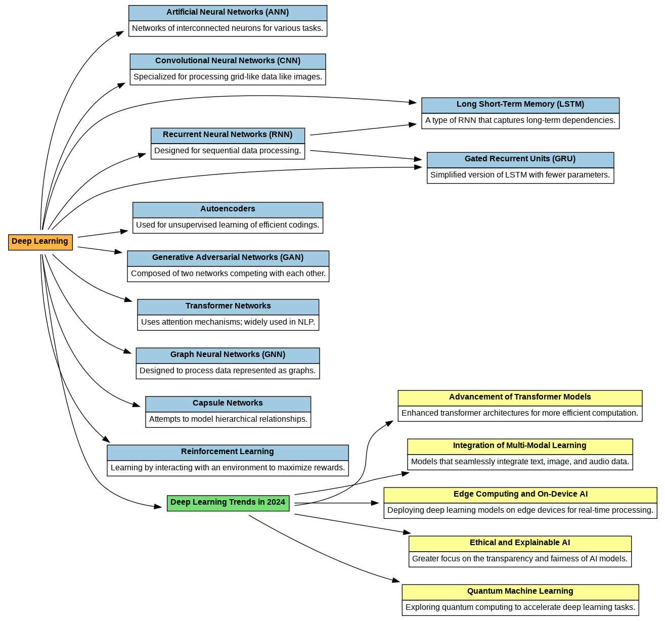
Understanding Convolutional Neural Networks (CNNs): A Step-by-Step Breakdown Convolutional Neural Networks (CNNs) are widely used in deep learning due to their ability to efficiently process image data. They perform complex operations on input images, enabling tasks like image classification, object detection, and segmentation. This step-by-step guide explains each stage of a CNN’s process, along with an example to clarify the concepts. 1. Input Image Representation The first step is providing an image to the network as input. Typically, the image is represented as a 3D matrix where the dimensions are: Height: Number of pixels vertically. Width: Number of pixels horizontally. Channels: Number of color channels (e.g., RGB for color images). Example: A 32×32 RGB image is represented with the shape: (32, 32, 3) 2. Convolutional Layer The Convolutional Layer applies filters to the image. Filters are small matrices that slide over the image, performing element-wise multiplication followed by summation. This produces feature maps. Each filter detects specific features like edges or textures. The network learns these filters during training. Mathematical Operation: 3. Activation Function (ReLU) After the convolutional layer, an Activation Function is applied. The most common activation function is ReLU (Rectified Linear Unit), which is mathematically expressed as: ReLU...

Membership Required

You must be a member to access this content.

View Membership Levels

Already a member? Log in here

Deep Learning Models integration for iOS Apps – briefly explained – Day 52

Key Deep Learning Models for iOS Apps Natural Language Processing (NLP) Models NLP models enable apps to understand and generate human-like text, supporting features like chatbots, sentiment analysis, and real-time translation. Top NLP Models for iOS: • Transformers (e.g., GPT, BERT, T5): Powerful for text generation, summarization, and answering queries. • Llama: A lightweight, open-source alternative to GPT, ideal for mobile apps due to its resource efficiency. Example Use Cases: • Building chatbots with real-time conversational capabilities. • Developing sentiment analysis tools for analyzing customer feedback. • Designing language translation apps for global users. Integration Tools: • Hugging Face: Access pre-trained models like GPT, BERT, and Llama for immediate integration. • PyTorch: Fine-tune models and convert them to Core ML for iOS deployment. Generative AI Models Generative AI models create unique content, including text, images, and audio, making them crucial for creative apps. Top Generative AI Models: • GANs (Generative Adversarial Networks): Generate photorealistic images, videos, and audio. • Llama with Multimodal Extensions: Handles both text and images efficiently, ideal for creative applications. • VAEs (Variational Autoencoders): Useful for reconstructing data and personalization. Example Use Cases: • Apps for generating digital art and music. • Tools for personalized content creation,...

Membership Required

You must be a member to access this content.

View Membership Levels

Already a member? Log in here
InSight Media Briefing (NHQ201810310009)

Deep Learning Examples, Short OverView – Day 51

Deep Learning Guide Comprehensive Guide to Deep Learning in 2024 and 2025: Trends, Types, and Beginner Tips Deep learning continues to be at the forefront of advancements in artificial intelligence (AI), shaping industries across the globe, from healthcare and finance to entertainment and retail. With its ability to learn from vast datasets, deep learning has become a key driver of innovation. As we look to 2024 and 2025, deep learning is poised for even greater leaps forward. In this comprehensive guide, we’ll explore the types of deep learning models, the latest trends shaping the field, and beginner-friendly tips to get started. _Examples of Types of Deep Learning Models_ Deep learning is a subset of machine learning that uses neural networks with many layers to analyze and interpret complex data patterns. These networks are inspired by the human brain and can be trained to recognize patterns, make predictions, and perform various tasks with minimal human intervention. In 2024 and 2025, deep learning will play an increasingly critical role in powering applications across sectors like healthcare, autonomous systems, natural language processing, and more. _Examples of Types of Deep Learning Models_   Feedforward Neural Networks (FNNs) Description: FNNs are the simplest form of...

Membership Required

You must be a member to access this content.

View Membership Levels

Already a member? Log in here

Deep Neural Networks vs Dense Network – Day 50

Deep Neural Networks (DNNs) vs Dense Networks Understanding the distinction between Deep Neural Networks (DNNs) and Dense Networks is crucial for selecting the appropriate architecture for your machine learning or deep learning tasks. Deep Neural Networks (DNNs) Definition: A Deep Neural Network is characterized by multiple layers between the input and output layers, enabling the model to learn complex patterns and representations from data. Key Characteristics: Composed of several hidden layers, each transforming the input data into more abstract representations. Can include various types of layers, such as convolutional layers for image data or recurrent layers for sequential data. When to Use: Ideal for tasks involving unstructured data like images, text, or audio. Suitable for applications requiring the capture of intricate patterns, such as image recognition, natural language processing, and speech recognition. Dense Networks Definition: A Dense Network, also known as a fully connected network, is a type of neural network layer where each neuron is connected to every neuron in the preceding layer. Key Characteristics: Each neuron receives input from all neurons in the previous layer, allowing for comprehensive learning of data relationships. Often used in the final stages of a neural network to integrate features learned in previous...

Membership Required

You must be a member to access this content.

View Membership Levels

Already a member? Log in here
letter blocks

Learn Max-Norm Regularization to avoid overfitting : Theory and Importance in Deep Learning and proof – Day 49

Max-Norm Regularization: Theory and Importance in Deep Learning Introduction Max-norm regularization is a weight constraint technique used in deep learning to prevent the weights of a neural network from growing too large. This method helps prevent overfitting by ensuring that the model doesn’t rely too heavily on specific features by excessively growing weights. Instead, max-norm regularization constrains the weight vector so that its size remains manageable, which stabilizes training and improves the model’s ability to generalize to new data. This technique is particularly useful in deep networks like Convolutional Neural Networks (CNNs) and Recurrent Neural Networks (RNNs), where large weights can cause significant problems such as unstable gradients or overfitting during training. 1. Why Regularization is Needed in Neural Networks Neural networks are flexible models capable of learning complex relationships between inputs and outputs. However, this flexibility can lead to overfitting, where the model memorizes the training data rather than learning general patterns. One key reason for overfitting is the uncontrolled growth of large weights during training. When weights grow too large, the model becomes too sensitive to small variations in input, causing unstable predictions and poor generalization on unseen data. Regularization methods like max-norm regularization directly address this issue...

Membership Required

You must be a member to access this content.

View Membership Levels

Already a member? Log in here

DropOut and Monte Carlo Dropout (MC Dropout)- Day 48

Understanding Dropout in Neural Networks Understanding Dropout in Neural Networks with a Real Numerical Example In deep learning, overfitting is a common problem where a model performs extremely well on training data but fails to generalize to unseen data. One popular solution is dropout, which randomly deactivates neurons during training, making the model more robust. In this section, we will demonstrate dropout with a simple example using numbers and explain how dropout manages weights during training. What is Dropout? Dropout is a regularization technique used in neural networks to prevent overfitting. In a neural network, neurons are connected between layers, and dropout randomly turns off a subset of those neurons during the training phase. When dropout is applied, each neuron has a probability \( p \) of being “dropped out” (i.e., set to zero). For instance, if \( p = 0.5 \), each neuron has a 50% chance of being dropped for a particular training iteration. Importantly, dropout does not remove neurons or weights permanently. Instead, it temporarily deactivates them during training, and they may be active again in future iterations.   Let’s walk through a numerical example to see how dropout works in action and how weights are managed...

Membership Required

You must be a member to access this content.

View Membership Levels

Already a member? Log in here

Understanding Regularization in Deep Learning – Day 47

Understanding Regularization in Deep Learning – A Mathematical and Practical Approach Introduction One of the most compelling challenges in machine learning, particularly with deep learning models, is overfitting. This occurs when a model performs exceptionally well on the training data but fails to generalize to unseen data. Regularization offers solutions to this issue by controlling the complexity of the model and preventing it from overfitting. In this post, we’ll explore the different types of regularization techniques—L1, L2, and dropout—diving into their mathematical foundations and practical implementations. What is Overfitting? In machine learning, a model is said to be overfitting when it learns not just the actual patterns in the training data but also the noise and irrelevant details. While this enables the model to perform well on training data, it results in poor performance on new, unseen data. The flexibility of neural networks, with their vast number of parameters, makes them highly prone to overfitting. This flexibility allows them to model very complex relationships in the data, but without precautions, they end up memorizing the training data instead of generalizing from it. Regularization is the key to addressing this challenge. L1 and L2 Regularization: The Mathematical Backbone L1 Regularization (Lasso...

Membership Required

You must be a member to access this content.

View Membership Levels

Already a member? Log in here

Comparing TensorFlow (Keras), PyTorch, & MLX – Day 46

  Comparing Deep Learning on TensorFlow (Keras), PyTorch, and Apple’s MLX Deep learning frameworks such as TensorFlow (Keras), PyTorch, and Apple’s MLX offer powerful tools to build and train machine learning models. Despite solving similar problems, these frameworks have different philosophies, APIs, and optimizations under the hood. In this post, we will examine how the same model is implemented on each platform and why the differences in code arise, especially focusing on why MLX is more similar to PyTorch than TensorFlow. 1. Model in PyTorch PyTorch is known for giving developers granular control over model-building and training processes. The framework encourages writing custom training loops, making it highly flexible, especially for research purposes. PyTorch Code: What’s Happening Behind the Scenes in PyTorch? PyTorch gives the developer direct control over every step of the model training process. The training loop is written manually, where: Forward pass: Defined in the forward() method, explicitly computing the output layer by layer. Backward pass: After calculating the loss, the gradients are computed using loss.backward(). Gradient updates: The optimizer manually updates the weights after each batch using optimizer.step(). This manual training loop allows researchers and developers to experiment with unconventional architectures or optimization methods. The gradient...

Membership Required

You must be a member to access this content.

View Membership Levels

Already a member? Log in here

Learning Rate – 1-Cycle Scheduling, exponential decay and Cyclic Exponential Decay (CED) – Part 4 – Day 45

Advanced Learning Rate Scheduling Methods for Machine Learning: Learning rate scheduling is critical in optimizing machine learning models, helping them converge faster and avoid pitfalls such as getting stuck in local minima. So far in our pervious days articles we have explained a lot about optimizers, learning rate schedules, etc. In this guide, we explore three key learning rate schedules: Exponential Decay, Cyclic Exponential Decay (CED), and 1-Cycle Scheduling, providing mathematical proofs, code implementations, and theory behind each method. 1. Exponential Decay Learning Rate Exponential Decay reduces the learning rate by a factor of , allowing larger updates early in training and smaller, more refined updates as the model approaches convergence. Formula: Where: is the learning rate at time step , is the initial learning rate, is the decay rate, controlling how fast the learning rate decreases, represents the current time step (or epoch). Mathematical Proof of Exponential Decay The core idea of exponential decay is that the learning rate decreases over time. Let’s prove that this results in convergence. The parameter update rule for gradient descent is: Substituting the exponentially decayed learning rate: As , the decay factor , meaning that the updates to become smaller and smaller, allowing...

Membership Required

You must be a member to access this content.

View Membership Levels

Already a member? Log in here

Exploring Gradient Clipping & Weight Initialization in Deep Learning – Day 44

Understanding Gradient Clipping and Weight Initialization Techniques in Deep Learning In this part, we explore the fundamental techniques of gradient clipping and weight initialization in more detail. Both of these methods play a critical role in ensuring deep learning models train efficiently and avoid issues like exploding or vanishing gradients. Gradient Clipping: Controlling Exploding Gradients When training deep learning models, especially very deep or recurrent neural networks (RNNs), one of the main challenges is dealing with exploding gradients. This happens when the gradients (which are used to update the model’s weights) grow too large during backpropagation, causing unstable training or even model failure. Gradient clipping is a method used to limit the magnitude of the gradients during training. Here’s how it works and why it’s useful: How Gradient Clipping Works: During backpropagation, the gradients are calculated for each parameter. If a gradient exceeds a predefined threshold, it is scaled down to fit within that threshold. There are two main types of gradient clipping: Norm-based clipping: The magnitude (norm) of the entire gradient vector is computed. If the norm exceeds the threshold, the gradients are scaled down proportionally. Value-based clipping: If any individual gradient component exceeds a set value, that specific...

Membership Required

You must be a member to access this content.

View Membership Levels

Already a member? Log in here