small update for MLX user of apple – M4 Chips is coming
Apple Releases MacBook Pro with M4 Chip in 2024 Apple Announces New MacBook Pro with M4 Chip Posted on October 4, 2024 by Admin What […]
Apple Releases MacBook Pro with M4 Chip in 2024 Apple Announces New MacBook Pro with M4 Chip Posted on October 4, 2024 by Admin What […]
A Deep Dive into Recurrent Neural Networks, Layer Normalization, and LSTMs So far we have explained in pervious days articles a lot about RNN. We have explained, Recurrent Neural Networks (RNNs) are a cornerstone in handling sequential data, ranging from time series analysis to natural language processing. However, training RNNs comes with challenges, particularly when dealing with long sequences and issues like unstable gradients. This post will cover how Layer Normalization (LN) addresses these challenges and how Long Short-Term Memory (LSTM) networks provide a more robust solution to memory retention in sequence models. The Challenges of RNNs: Long Sequences and...
Mastering Time Series Forecasting with RNNs and Seq2Seq Models: Detailed Iterations with Calculations, Tables, and Method-Specific Features Time series forecasting is a crucial task in various domains such as finance, weather prediction, and energy management. Recurrent Neural Networks (RNNs) and Sequence-to-Sequence (Seq2Seq) models are powerful tools for handling sequential data. In this guide, we will provide step-by-step calculations, including forward passes, loss computations, and backpropagation for two iterations across three forecasting methods: Assumptions and Initial Parameters For consistency across all methods, we’ll use the following initial parameters: 1. Iterative Forecasting: Predicting One Step at a Time In iterative forecasting, the...
Step-by-Step Explanation of RNN for Time Series Forecasting Step 1: Simple RNN for Univariate Time Series Forecasting Explanation: An RNN processes sequences of data, where the output at any time step depends on both the current input and the hidden state (which stores information about previous inputs). In this case, we use a Simple RNN with only one recurrent neuron. TensorFlow Code: Numerical Example: Let’s say we have a sequence of three time steps: . 1. Input and Hidden State Initialization: The RNN starts with an initial hidden state , typically initialized to 0. Each step processes the input and...
A Deep Dive into ARIMA, SARIMA, and Their Relationship with Deep Learning for Time Series Forecasting In recent years, deep learning has become a dominant force in many areas of data analysis, and time series forecasting is no exception. Traditional models like ARIMA (Autoregressive Integrated Moving Average) and its seasonal extension SARIMA have long been the go-to solutions for forecasting time-dependent data. However, newer models based on Recurrent Neural Networks (RNNs), particularly Long Short-Term Memory (LSTM) networks, have emerged as powerful alternatives. Both approaches have their strengths and applications, and understanding their relationship helps in choosing the right tool for...
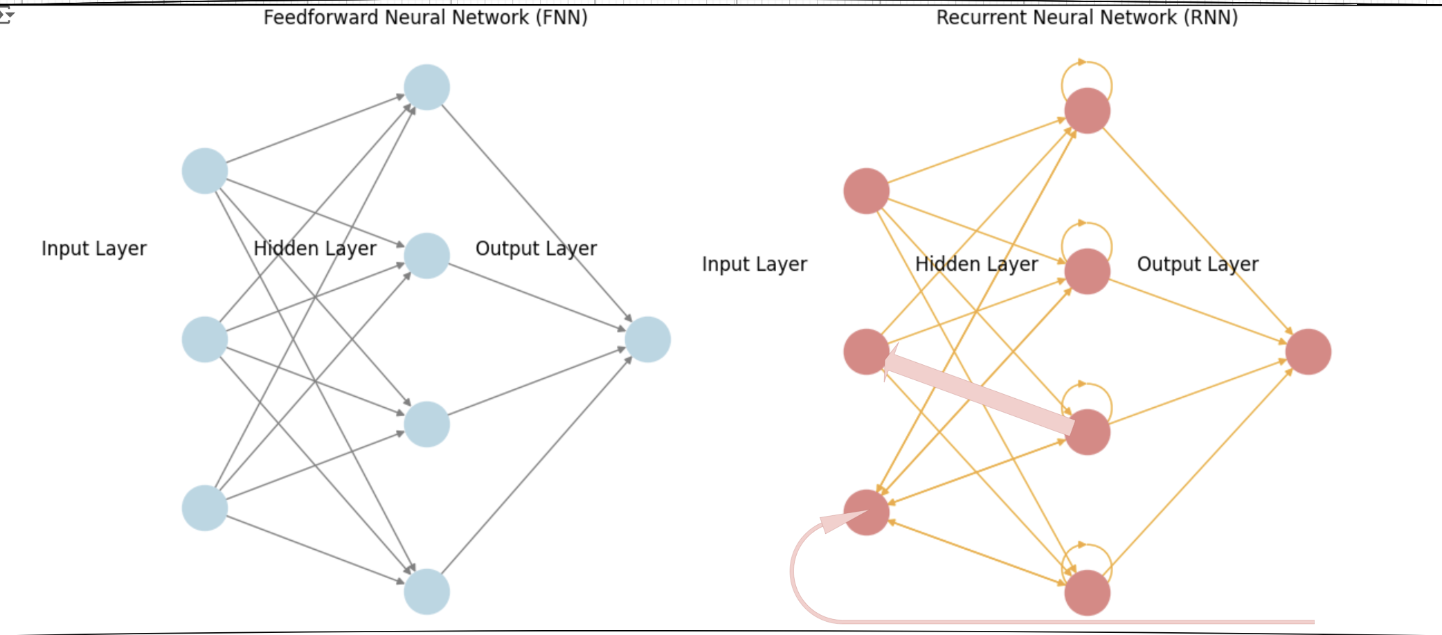
In this article we try to show an example of FNN and for RNN TO understand the math behind it better by comparing to each other: Neural Networks Example Example Setup 1. Feedforward Neural Network (FNN) Structure Input Layer: 1 neuron Hidden Layer: 1 neuron Output Layer: 1 neuron Weights and Biases Initial Weights: (Input to Hidden weight) (Hidden to Output weight) Biases: (Hidden layer bias) (Output layer bias) Step-by-Step Calculation for FNN Step 1: Forward Pass Hidden Layer Output: Output: Step 2: Loss Calculation Using Mean Squared Error (MSE): Step 3: Backward Pass Gradient of Loss with respect...
Time Series Forecasting with Recurrent Neural Networks (RNNs): A Complete Guide Introduction Time series data is all around us: from stock prices and weather patterns to daily ridership on public transport systems. Accurately forecasting future values in a time series is a challenging task, but Recurrent Neural Networks (RNNs) have proven to be highly effective at this. In this article, we will explore how RNNs can be applied to time series forecasting, explain the key concepts behind them, and demonstrate how to clean, prepare, and visualize time series data before feeding it into an RNN. What Is a Recurrent Neural...
Understanding Recurrent Neural Networks (RNNs) Recurrent Neural Networks (RNNs) are a class of neural networks that excel in handling sequential data, such as time series, text, and speech. Unlike traditional feedforward networks, RNNs have the ability to retain information from previous inputs and use it to influence the current output, making them extremely powerful for tasks where the order of the input data matters. In day 55 article we have introduced RNN. In this article, we will explore the inner workings of RNNs, break down their key components, and understand how they process sequences of data through time. We’ll also...
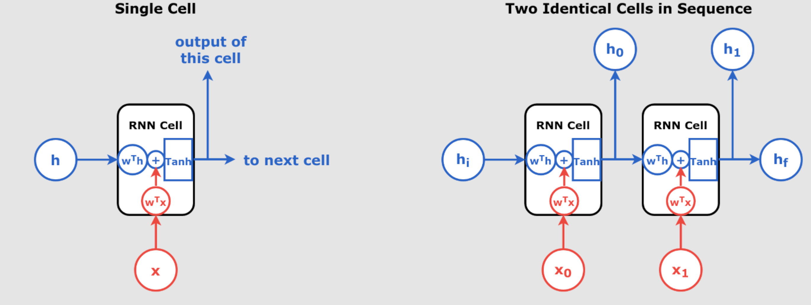
Understanding Recurrent Neural Networks (RNNs) and CNNs for Sequence Processing Introduction In the world of deep learning, neural networks have become indispensable, especially for handling tasks involving sequential data, such as time series, speech, and text. Among the most popular architectures for such data are Recurrent Neural Networks (RNNs) and Convolutional Neural Networks (CNNs). Although RNNs are traditionally associated with sequence processing, CNNs have also been adapted to perform well in this area. This blog will take a detailed look at how these networks work, their differences, their challenges, and their real-world applications. Unrolling RNNs: How RNNs Process Sequences One...
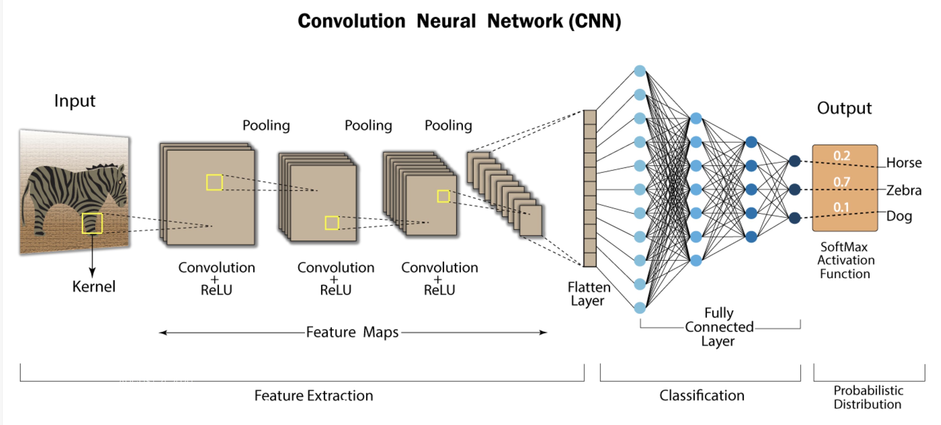
You have seen what CNNs are in our previous article. [View Article] Now, let’s explore the mathematics behind CNNs in detail, step by step, with a very simple example. Part 1: Input Layer, Convolution, and Pooling (Steps 1-4) Step 1: Input Layer We are processing two 3×3 grayscale images—one representing a zebra and one representing a cat. Image 1: Zebra Image (e.g., with stripe-like patterns) Image 2: Cat Image (e.g., with smoother, fur-like textures) These images are represented as 2D grids of pixel values, with each value between 0 and 1 indicating pixel intensity. Step 2: Convolutional Layer (Feature Extraction)...


For best results, phrase your question similar to our FAQ examples.