Reinforcement Learning: An Evolution from Games to Real-World Impact

Reinforcement Learning (RL) is a fascinating branch of machine learning, with its roots stretching back to the 1950s. Although not always in the limelight, RL made a significant impact in various domains, especially in gaming and machine control. In 2013, a team from DeepMind, a British startup, built a system capable of learning and excelling at Atari games using only raw pixels as input—without any knowledge of the game’s rules. This breakthrough led to DeepMind’s famous system, AlphaGo, defeating world Go champions and ignited a global interest in RL.

The Foundations of Reinforcement Learning: How It Works

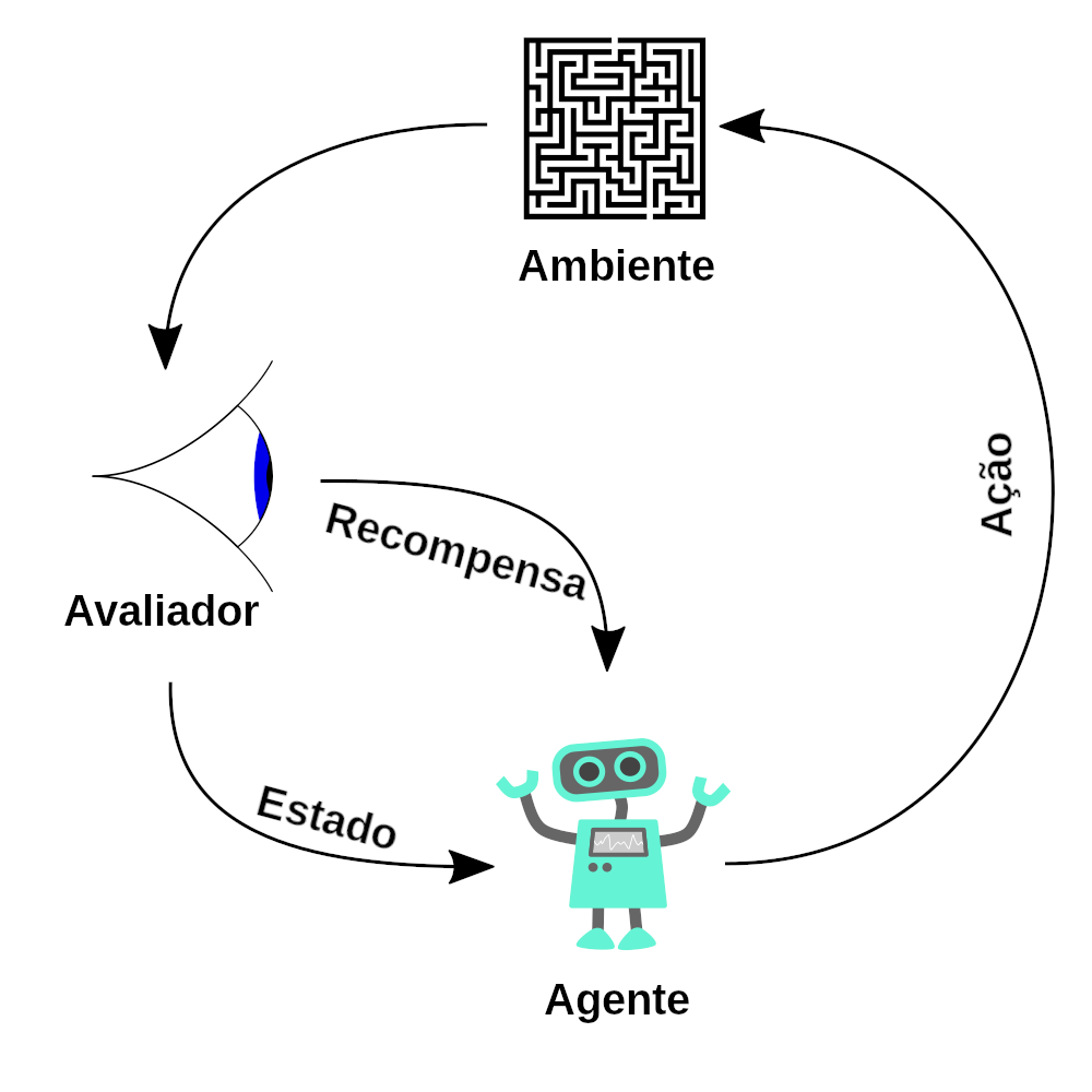
In RL, an agent interacts with an environment, observes outcomes, and receives feedback through rewards. The agent’s objective is to maximize cumulative rewards over time, learning the best actions through trial and error.

Term	Explanation
Agent	The software or system making decisions.
Environment	The external setting with which the agent interacts.
Reward	Feedback from the environment based on the agent’s actions.

Examples of RL Applications

Here are a few tasks RL is well-suited for:

Application	Agent	Environment	Reward
Robot Control	Robot control program	Real-world physical space	Positive for approaching target, negative for incorrect movement
Atari Game	Game-playing program	Game simulation	Points scored in the game
Board Game (e.g., Go)	Game-playing program	Game board	Reward only if it wins the game
Smart Thermostat	Thermostat control program	Indoor temperature settings	Positive for saving energy, negative if adjustments are needed by humans
Stock Market	Trading agent	Financial market data	Monetary gains and losses

Defining Policy: The Agent’s Guide to Action

The approach or “policy” an agent uses to decide its actions is central to RL. A policy can be as straightforward as a set of if-then rules or as complex as a deep neural network that analyzes observations to output actions. Policies can be deterministic or stochastic (random). In training an agent, policy search methods help identify effective policies, often through trial and error.

Policy Search and Optimization Techniques

Method	Description
Brute-Force Search	Tries various policy parameters systematically, though it’s not feasible for complex policies.
Genetic Algorithms	Generates multiple policies, selects the best, and iterates through generations with random mutations.
Policy Gradients (PG)	Adjusts policy parameters by evaluating gradients based on rewards to optimize actions.

Getting Started with OpenAI Gym

Training RL agents requires environments where the agent can safely learn and test its policies. OpenAI Gym is a popular toolkit that offers simulated environments for RL training, from Atari games to physical simulations. By using OpenAI Gym, developers can safely experiment and refine RL agents without needing a physical setup.

Setting Up OpenAI Gym

To install and use OpenAI Gym on Colab or a local machine, developers can use the following commands:

# Upgrade Gym and install dependencies on Colab
%pip install -q -U gym
%pip install -q -U gym[classic_control,box2d,atari,accept-rom-license]

These commands install Gym and essential libraries for running classic and Atari environments.

Creating a CartPole Environment

In this 2D environment, a cart must balance a pole by deciding when to move left or right:

import gym
env = gym.make("CartPole-v1", render_mode="rgb_array")
obs, info = env.reset(seed=42)
print(obs)  # Initial observation

Here, obs is a 1D array representing the cart’s position and velocity, as well as the pole’s angle and angular velocity.

Observation	Description
Horizontal Position	Cart’s position relative to the center (0.0 = center).
Velocity	Speed and direction of the cart.
Angle	Pole’s tilt relative to vertical (0.0 = perfectly vertical).
Angular Velocity	Speed and direction of the pole’s tilt.

Implementing a Simple Policy for CartPole

This policy directs the cart to move left or right based on the pole’s tilt angle:

def basic_policy(obs):
    angle = obs[2]
    return 0 if angle < 0 else 1

The policy adjusts based on the observation, keeping the pole balanced for as long as possible. After running multiple trials, we can evaluate its performance:

totals = []
for episode in range(500):
    episode_rewards = 0
    obs, info = env.reset(seed=episode)
    for step in range(200):
        action = basic_policy(obs)
        obs, reward, done, truncated, info = env.step(action)
        episode_rewards += reward
        if done or truncated:
            break
    totals.append(episode_rewards)

The results, such as the mean and standard deviation of rewards, indicate how well this simple policy performs.

Mathematic behind Reinforecement

The RL Loop

At the core of RL is the interaction between the agent and the environment.

+---------+       Action        +-------------+
|         | --------------->    |             |
|  Agent  |                     | Environment |
|         |    <--------------- |             |
+---------+    Observation      +-------------+
                   (State, Reward)

Figure 1: The Agent-Environment Interaction Loop

Agent: Learns and decides which action to take.
Environment: Responds to the agent's actions and provides feedback.

Markov Decision Processes (MDPs)

An MDP provides a mathematical framework for modeling RL problems.

Components of an MDP

States (S): All possible situations the agent can be in.
Actions (A): All possible moves the agent can make.
Transition Probability (P): Probability of moving from one state to another given an action.
Reward Function (R): Feedback received after taking an action.
Discount Factor (γ): Determines the importance of future rewards.

Value Functions and the Bellman Equations

Value functions estimate how good it is to be in a state or to perform an action in a state.

State-Value Function V^π(s)

$V^{\pi}(s) = \mathbb{E}_{\pi} \left[ \sum_{t=0}^{\infty} \gamma^t r_{t+1} \,|\, s_0 = s \right]$

$V^{\pi}(s)$ : Value of state $s$ under policy $\pi$ .

$\mathbb{E}_{\pi} [ \cdot ]$ : Expected value when following policy $\pi$ .

$\sum_{t=0}^{\infty}$ : Sum over all future time steps.

$\gamma^t$ : Discount factor raised to the power $t$ (0 ≤ $\gamma$ ≤ 1).

$r_{t+1}$ : Reward at time $t+1$ .

$s_0 = s$ : Starting from state $s$ at time $t = 0$ .

Action-Value Function $Q^{\pi}(s, a)$

$Q^{\pi}(s, a) = \mathbb{E}_{\pi} \left[ \sum_{t=0}^{\infty} \gamma^t r_{t+1} \,|\, s_0 = s, a_0 = a \right]$

$Q^{\pi}(s, a)$ : Value of taking action $a$ in state $s$ under policy $\pi$ .

$a_0 = a$ : Taking action $a$ at the initial time.

Other terms are as previously defined.

The Bellman Expectation Equation

For the state-value function:

$V^{\pi}(s) = \sum_{a \in A} \pi(a | s) \sum_{s' \in S} P(s' | s, a) \left[ R(s, a) + \gamma V^{\pi}(s') \right]$

$V^{\pi}(s)$ : Value of state $s$ under policy $\pi$ .

$\pi(a | s)$ : Probability of taking action $a$ in state $s$ under policy $\pi$ .

$P(s' | s, a)$ : Probability of transitioning to state $s'$ from $s$ after action $a$ .

$R(s, a)$ : Immediate reward after action $a$ in state $s$ .

$V^{\pi}(s')$ : Value of the next state $s'$ .

Q-Learning and Temporal Difference Learning

Q-Learning is a model-free RL algorithm that seeks to learn the optimal policy.

Q-Learning Update Rule

$Q(s_t, a_t) \leftarrow Q(s_t, a_t) + \alpha \left[ r_{t+1} + \gamma \max_{a'} Q(s_{t+1}, a') - Q(s_t, a_t) \right]$

$Q(s_t, a_t)$ : Current estimate of the Q-value for state $s_t$ and action $a_t$ .

$\leftarrow$ : Update operation; assigns the new value to $Q(s_t, a_t)$ .

$\alpha$ : Learning rate ( $0 < \alpha \leq 1$ ).

$r_{t+1}$ : Reward received after taking action $a_t$ .

$\gamma$ : Discount factor.

$\max_{a'} Q(s_{t+1}, a')$ : Maximum estimated Q-value for the next state $s_{t+1}$ over all possible actions $a'$ .

$Q(s_t, a_t)$ : Current Q-value before the update.

Q-Learning Variables

Table 1: Q-Learning Variables
Symbol	Description
$s_t$	Current state
$a_t$	Action taken at state $s_t$
$r_{t+1}$	Reward received after action $a_t$
$s_{t+1}$	Next state after action $a_t$
$\alpha$	Learning rate
$\gamma$	Discount factor
$Q(s_t, a_t)$	Current Q-value estimate

Function Approximation with Neural Networks

When dealing with large or continuous state spaces, we use neural networks to approximate the Q-function.

Neural Network Approximation

[Input Layer]: State s_t
        |
[Hidden Layers]
        |
[Output Layer]: Q-values for all actions

Figure 2: Neural Network Approximation

Input: State representation.
Output: Estimated Q-values for possible actions.

Deep Q-Networks (DQN)

DQN combines Q-Learning with deep neural networks.

Key Components of DQN

Experience Replay: Stores agent's experiences and samples mini-batches to break correlation.
Target Network: A separate network to calculate target Q-values, improving stability.

DQN Loss Function

$L(\theta) = \mathbb{E}_{(s, a, r, s')} \left[ \left( y - Q(s, a; \theta) \right)^2 \right]$

$L(\theta)$ : Loss function to minimize during training.

$\mathbb{E}_{(s, a, r, s')} \left[ \cdot \right]$ : Expected value over the experience replay buffer containing tuples $(s, a, r, s')$ .

$y$ : Target Q-value.

$Q(s, a; \theta)$ : Predicted Q-value from the network for state $s$ and action $a$ , parameterized by $\theta$ .

Where the target Q-value $y$ is:

$y = r + \gamma \max_{a'} Q(s', a'; \theta^-)$

$y$ : Target Q-value.

$r$ : Reward received after taking action $a$ in state $s$ .

$\gamma$ : Discount factor.

$\max_{a'} Q(s', a'; \theta^-)$ : Maximum predicted Q-value for the next state $s'$ over all actions $a'$ , using the target network parameters $\theta^-$ .

$\theta^-$ : Parameters of the target network (a delayed copy of $\theta$ ).

Policy Gradient Methods

Policy Gradient methods optimize the policy directly.

Policy Representation

$\pi_{\theta}(a\,|\,s)$ : Probability of taking action $a$ in state $s$ , parameterized by $\theta$ .

Objective Function

$J(\theta) = \mathbb{E}_{\pi_{\theta}} \left[ \sum_{t=0}^{\infty} \gamma^t \, r_{t+1} \right]$

$J(\theta)$ : Performance measure of the policy.

$\mathbb{E}_{\pi_{\theta}} \left[ \cdot \right]$ : Expected reward under the policy $\pi_{\theta}$ .

$\gamma^t$ : Discount factor raised to the power $t$ .

$r_{t+1}$ : Reward received at time $t+1$ .

Actor-Critic Algorithms

Actor-Critic algorithms combine policy-based and value-based methods to improve stability and efficiency.

Actor Update

$\theta_{\text{actor}} \leftarrow \theta_{\text{actor}} + \alpha_{\text{actor}} \cdot \delta_t \cdot \nabla_{\theta_{\text{actor}}} \log \pi_{\theta_{\text{actor}}}(a_t\,|\,s_t)$

$\theta_{\text{actor}}$ : Parameters of the actor (policy) network.

$\alpha_{\text{actor}}$ : Learning rate for the actor network.

$\delta_t$ : Temporal Difference (TD) error calculated as:

$\delta_t = r_{t+1} + \gamma V_{\theta_{\text{critic}}}(s_{t+1}) - V_{\theta_{\text{critic}}}(s_t)$

$\nabla_{\theta_{\text{actor}}} \log \pi_{\theta_{\text{actor}}}(a_t\,|\,s_t)$ : Gradient of the log-probability of the action taken with respect to the actor’s parameters.

Critic Update

$\theta_{\text{critic}} \leftarrow \theta_{\text{critic}} + \alpha_{\text{critic}} \cdot \delta_t \cdot \nabla_{\theta_{\text{critic}}} V_{\theta_{\text{critic}}}(s_t)$

$\theta_{\text{critic}}$ : Parameters of the critic (value function) network.

$\alpha_{\text{critic}}$ : Learning rate for the critic network.

$\delta_t$ : Temporal Difference error (as calculated above).

$\nabla_{\theta_{\text{critic}}} V_{\theta_{\text{critic}}}(s_t)$ : Gradient of the value function estimate with respect to the critic's parameters.

Advanced Techniques in Deep RL

Recent advances in RL leverage complex algorithms and architectures to improve performance in challenging environments.

Proximal Policy Optimization (PPO)

PPO improves training stability by limiting the extent to which policy updates can deviate. It applies a clipping function to the policy loss, constraining how much the updated policy can differ from the old policy.

Soft Actor-Critic (SAC)

SAC introduces an entropy term into the reward function, encouraging exploration by making the agent seek stochastic policies. The objective is to maximize both the reward and the policy’s entropy.

Applications of RL with Neural Networks

Gaming

AlphaGo: Used RL to achieve superhuman performance in the game of Go by combining deep neural networks with Monte Carlo tree search.
Atari Games: Achieved human-level performance on many Atari games using DQN, which learns directly from raw pixel inputs.

Robotics

Manipulation: RL helps robots learn to pick and manipulate objects with precision.
Locomotion: Agents use RL to learn movement patterns for walking, running, and navigating through obstacles.

Autonomous Vehicles

Navigation: RL helps autonomous vehicles make real-time decisions in complex, dynamic environments.

Conclusion

Reinforcement learning, especially when combined with neural networks, has transformed the field of AI, enabling machines to tackle complex tasks across multiple domains. Understanding the mathematical foundations and practical applications of RL helps us appreciate its potential and limitations as we continue to explore its capabilities in the real world.

Step

Concept

Details

Markov Decision Processes (MDP)

An MDP provides a mathematical framework for modeling decision-making where outcomes are partly random and partly under the control of a decision-maker.

Symbol	Description
$S$	Set of all possible states
$A$	Set of all possible actions
$P(s'\|s, a)$	Probability of transitioning to state $s'$ from state $s$ after taking action $a$
$R(s, a)$	Expected reward received after taking action $a$ in state $s$
$\gamma$	Discount factor, $0 \leq \gamma \leq 1$ , which determines the importance of future rewards

Markov Property: The future state depends only on the current state and action, not on the sequence of events that preceded it.

Value Functions

Value functions estimate how good it is to be in a given state or to perform a specific action in a state, in terms of expected return (cumulative future rewards).

Function	Definition
State-Value Function $V^\pi(s)$	$V^\pi(s) = \mathbb{E}_\pi \left[ \sum_{t=0}^\infty \gamma^t R(s_t, a_t) \,\bigg\|\, s_0 = s \right]$ This represents the expected return starting from state $s$ , and following policy $\pi$ thereafter.
Action-Value Function $Q^\pi(s, a)$	$Q^\pi(s, a) = \mathbb{E}_\pi \left[ \sum_{t=0}^\infty \gamma^t R(s_t, a_t) \,\bigg\|\, s_0 = s, a_0 = a \right]$ This represents the expected return starting from state $s$ , taking action $a$ , and thereafter following policy $\pi$ .

Explanation: The expectation $\mathbb{E}_\pi$ is taken over all possible sequences of future states and actions, weighted by the probability of their occurrence under policy $\pi$ . The discount factor $\gamma$ reduces the weight of future rewards exponentially, ensuring the sum converges for infinite horizons.

Bellman Equations

The Bellman equations provide recursive definitions for the value functions, expressing the value of a state (or state-action pair) in terms of the immediate reward and the value of successor states.

Equation	Description
$V^\pi(s) = \sum_{a} \pi(a\|s) \left[ R(s, a) + \gamma \sum_{s'} P(s'\|s, a) V^\pi(s') \right]$	Bellman Expectation Equation for the State-Value Function. Explanation: The value of state $s$ under policy $\pi$ is the expected value of the immediate reward $R(s, a)$ plus the discounted value of the next state $V^\pi(s')$ , averaged over all possible actions $a$ and successor states $s'$ .
$Q^\pi(s, a) = R(s, a) + \gamma \sum_{s'} P(s'\|s, a) \sum_{a'} \pi(a'\|s') Q^\pi(s', a')$	Bellman Expectation Equation for the Action-Value Function. Explanation: The value of taking action $a$ in state $s$ is the immediate reward plus the expected discounted value of the next state-action pair, where the next action $a'$ is chosen according to policy $\pi$ .

Optimal Value Functions and Policies

Optimal value functions represent the maximum expected return achievable from any state or state-action pair, under any policy.

Function	Definition
Optimal State-Value Function $V^*(s)$	$V^(s) = \max_\pi V^\pi(s)$ The highest expected return achievable from state $s$ by any policy.*
Optimal Action-Value Function $Q^*(s, a)$	$Q^(s, a) = \max_\pi Q^\pi(s, a)$ The highest expected return achievable from state $s$ and action $a$ by any policy.*

The Bellman Optimality Equations define these optimal value functions recursively:

Equation	Description
$V^(s) = \max_{a} \left[ R(s, a) + \gamma \sum_{s'} P(s'\|s, a) V^(s') \right]$	Bellman Optimality Equation for $V^(s)$ .* Explanation: The optimal value of state $s$ is the maximum expected return obtainable by choosing the best action $a$ , considering both the immediate reward and the discounted optimal value of the next state $s'$ .
$Q^(s, a) = R(s, a) + \gamma \sum_{s'} P(s'\|s, a) \max_{a'} Q^(s', a')$	Bellman Optimality Equation for $Q^(s, a)$ .* Explanation: The optimal value of taking action $a$ in state $s$ is the immediate reward plus the expected discounted optimal value of the best action $a'$ in the next state $s'$ .

Policies

A policy $\pi$ defines the agent's behavior by specifying the action to take in each state.

Type	Definition
Deterministic Policy	$\pi(s) = a$ Specifies a single action $a$ to take in state $s$ .
Stochastic Policy	$\pi(a\|s) = \mathbb{P}[A_t = a \,\|\, S_t = s]$ Gives a probability distribution over actions in state $s$ .

Policy Improvement: The process of improving a policy by making it greedy with respect to the current value function.

Temporal Difference (TD) Learning

TD learning methods update estimates based on a combination of observed rewards and existing estimates.

Term	Equation	Explanation
TD Error $\delta_t$	$\delta_t = R_{t+1} + \gamma V(S_{t+1}) - V(S_t)$	The difference between the predicted value and the observed value plus estimated value of the next state. - $R_{t+1}$ : Reward received after taking action at time $t$ . - $\gamma V(S_{t+1})$ : Discounted estimate of future value. - $V(S_t)$ : Current estimate of the value of state $S_t$ .
Value Update	$V(S_t) \leftarrow V(S_t) + \alpha \delta_t$	Adjusts the value estimate of state $S_t$ towards the target. - $\alpha$ : Learning rate, determining the step size of the update.

Q-Learning

Q-Learning is an off-policy TD control algorithm that aims to learn the optimal action-value function $Q^*(s, a)$ .

Update Rule	Equation	Explanation
Q-Value Update	$Q(S_t, A_t) \leftarrow Q(S_t, A_t) + \alpha \left[ R_{t+1} + \gamma \max_{a'} Q(S_{t+1}, a') - Q(S_t, A_t) \right]$	- Updates the estimate of $Q(S_t, A_t)$ using the reward $R_{t+1}$ and the maximum estimated future Q-value. - $\alpha$ : Learning rate. - $\gamma \max_{a'} Q(S_{t+1}, a')$ : Estimated optimal future value.

Explanation: The update rule adjusts the current Q-value towards the target, which is the immediate reward plus the discounted estimate of the optimal future Q-value.

Function Approximation & Neural Networks

In environments with large or continuous state spaces, it's impractical to maintain a table of Q-values. Function approximation methods, like neural networks, are used to estimate value functions.

Function Approximator	Equation
Q-function Approximation	$Q(s, a; \theta) \approx Q^*(s, a)$

Explanation: Here, $\theta$ represents the parameters (weights and biases) of the neural network that approximates the Q-function.

Deep Q-Networks (DQN)

DQN combines Q-learning with deep neural networks to handle high-dimensional state spaces.

Component	Equation	Explanation
Loss Function $L(\theta)$	$L(\theta) = \mathbb{E}_{s,a,r,s'} \left[ \left( y - Q(s, a; \theta) \right)^2 \right]$	- Measures the difference between the target Q-value $y$ and the estimated Q-value $Q(s, a; \theta)$ . - The expectation is over the experience replay buffer.
Target $y$	$y = r + \gamma \max_{a'} Q(s', a'; \theta^-)$	- $r$ : Immediate reward received after action $a$ in state $s$ . - $\gamma \max_{a'} Q(s', a'; \theta^-)$ : Estimated optimal future value using the target network parameters $\theta^-$ .

Explanation: The loss function quantifies how close the neural network's predictions are to the targets. The target network $\theta^-$ is a copy of the Q-network $\theta$ that is updated less frequently to stabilize learning.

Policy Gradient Methods

Policy gradient methods optimize the policy directly by adjusting its parameters to maximize expected return.

Component	Equation	Explanation
Objective Function $J(\theta)$	$J(\theta) = \mathbb{E}_\pi [ R ]$	- Represents the expected return when following policy $\pi$ parameterized by $\theta$ . - The goal is to find $\theta$ that maximizes $J(\theta)$ .
Policy Gradient	$\nabla_\theta J(\theta) = \mathbb{E}_\pi \left[ \nabla_\theta \log \pi_\theta(a\|s) Q^\pi(s, a) \right]$	- Provides the direction in parameter space to adjust $\theta$ to increase $J(\theta)$ . - $\nabla_\theta \log \pi_\theta(a\|s)$ : Gradient of the log-probability of action $a$ given state $s$ , with respect to $\theta$ . - $Q^\pi(s, a)$ : Expected return from state $s$ after taking action $a$ .

Explanation: By taking steps proportional to the policy gradient, we improve the policy to maximize expected rewards.

REINFORCE Algorithm

REINFORCE is a Monte Carlo policy gradient method that updates the policy based on complete episodes.

Gradient Estimate	$\nabla_\theta J(\theta) \approx \sum_{t=0}^T \nabla_\theta \log \pi_\theta(a_t\|s_t) G_t$
Update Rule	$\theta \leftarrow \theta + \alpha \nabla_\theta J(\theta)$

Explanation:

$G_t = \sum_{k=t}^T \gamma^{k-t} R_{k+1}$ is the return from time $t$ onward.
The gradient estimate sums over the episode, adjusting the policy parameters $\theta$ to increase the likelihood of actions that led to higher returns.
$\alpha$ is the learning rate.

Actor-Critic Methods

Actor-Critic methods combine the benefits of policy gradients and value function approximation.

Component	Equation	Explanation
TD Error $\delta_t$	$\delta_t = R_{t+1} + \gamma V(s_{t+1}; w) - V(s_t; w)$	- Measures the discrepancy between the predicted value and the actual reward plus estimated next value. - $V(s_t; w)$ : Estimated value of state $s_t$ using parameters $w$ .
Critic Update	$w \leftarrow w + \alpha_c \delta_t \nabla_w V(s_t; w)$	- Updates the critic's parameters $w$ to reduce the TD error. - $\alpha_c$ : Critic's learning rate.
Actor Update	$\theta \leftarrow \theta + \alpha_a \delta_t \nabla_\theta \log \pi(a_t\|s_t; \theta)$	- Updates the actor's parameters $\theta$ in the direction suggested by the TD error. - $\alpha_a$ : Actor's learning rate.

Explanation: The critic evaluates the current policy by estimating the value function, while the actor updates the policy parameters in a direction that improves performance according to the critic's feedback.

Mathematics Behind Neural Network Updates

Neural networks are trained by adjusting their parameters to minimize a loss function using gradient descent.

Update Rule	$\theta \leftarrow \theta - \alpha \nabla_\theta L(\theta)$

Explanation:

$L(\theta)$ : Loss function measuring the error between predicted and target values.
$\nabla_\theta L(\theta)$ : Gradient of the loss with respect to the parameters, computed using backpropagation.
$\alpha$ : Learning rate determining the step size in parameter space.
The negative sign indicates moving in the direction that minimizes the loss.

Example: DQN Update Step

Steps to update DQN parameters:

Sample Mini-batch: Sample transitions $(s_j, a_j, r_j, s'_j)$ from the replay buffer.
Compute Target: $y_j = r_j + \gamma \max_{a'} Q(s'_j, a'; \theta^-)$
Compute Loss: $L_j(\theta) = \left( y_j - Q(s_j, a_j; \theta) \right)^2$
Compute Gradients: $\nabla_\theta L_j(\theta) = -2 \left( y_j - Q(s_j, a_j; \theta) \right) \nabla_\theta Q(s_j, a_j; \theta)$
Update Parameters: $\theta \leftarrow \theta + \alpha \nabla_\theta L_j(\theta)$

Explanation:

By sampling a mini-batch, we break the correlation between sequential samples, improving training stability.
The target $y_j$ is computed using the target network parameters $\theta^-$ to stabilize learning.
The loss measures how close the network's Q-value predictions are to the target values.
Gradients are computed with respect to the network's parameters and used to update the network via gradient descent.

Exploration vs. Exploitation

Balancing the need to explore new actions to discover their value and exploiting known actions to maximize reward.

Method	Description
$\epsilon$ -Greedy Policy	- With probability $\epsilon$ , select a random action (exploration). - With probability $1 - \epsilon$ , select the action with the highest estimated Q-value (exploitation). - $\epsilon$ is often decayed over time to shift from exploration to exploitation as learning progresses.

Advanced Techniques

Enhancements to basic algorithms to improve performance and stability.

Double DQN: Addresses overestimation bias by decoupling the selection and evaluation of the action in the target computation.

$y = r + \gamma Q(s', \arg\max_{a'} Q(s', a'; \theta); \theta^-)$
Dueling DQN: Separates the estimation of the state value and the advantages of each action, improving learning efficiency.

$Q(s, a; \theta, \alpha, \beta) = V(s; \theta, \beta) + A(s, a; \theta, \alpha) - \frac{1}{|A|} \sum_{a'} A(s, a'; \theta, \alpha)$
Prioritized Experience Replay: Samples more important transitions (with higher TD errors) more frequently, focusing learning on significant experiences.

Summary

Reinforcement learning enables agents to learn optimal behaviors through interactions with an environment by maximizing cumulative rewards. The mathematical foundations, including MDPs, value functions, and Bellman equations, provide a framework for understanding and developing RL algorithms. Neural networks serve as powerful function approximators, especially in complex, high-dimensional environments, making advanced algorithms like DQN and policy gradient methods feasible.

Reinforcement Learning: An Evolution from Games to Real-World Impact – day 77

Reinforcement Learning: An Evolution from Games to Real-World Impact

The Foundations of Reinforcement Learning: How It Works

Examples of RL Applications

Defining Policy: The Agent’s Guide to Action

Policy Search and Optimization Techniques

Getting Started with OpenAI Gym

Setting Up OpenAI Gym

Creating a CartPole Environment

Implementing a Simple Policy for CartPole

The RL Loop

Markov Decision Processes (MDPs)

Components of an MDP

Value Functions and the Bellman Equations

State-Value Function V^π(s)

Action-Value Function $Q^{\pi}(s, a)$

The Bellman Expectation Equation

Q-Learning and Temporal Difference Learning

Q-Learning Update Rule

Q-Learning Variables

Function Approximation with Neural Networks

Neural Network Approximation

Deep Q-Networks (DQN)

Key Components of DQN

DQN Loss Function

Policy Gradient Methods

Policy Representation

Objective Function

Actor-Critic Algorithms

Actor Update

Critic Update

Advanced Techniques in Deep RL

Proximal Policy Optimization (PPO)

Soft Actor-Critic (SAC)

Applications of RL with Neural Networks

Gaming

Robotics

Autonomous Vehicles

Conclusion

don't miss our new posts. Subscribe for updates

Education

Reinforcement Learning: An Evolution from Games to Real-World Impact – day 77

Reinforcement Learning: An Evolution from Games to Real-World Impact

The Foundations of Reinforcement Learning: How It Works

Examples of RL Applications

Defining Policy: The Agent’s Guide to Action

Policy Search and Optimization Techniques

Getting Started with OpenAI Gym

Setting Up OpenAI Gym

Creating a CartPole Environment

Implementing a Simple Policy for CartPole

The RL Loop

Markov Decision Processes (MDPs)

Components of an MDP

Value Functions and the Bellman Equations

State-Value Function Vπ(s)

The Bellman Expectation Equation

Q-Learning and Temporal Difference Learning

Q-Learning Update Rule

Q-Learning Variables

Function Approximation with Neural Networks

Neural Network Approximation

Deep Q-Networks (DQN)

Key Components of DQN

DQN Loss Function

Policy Gradient Methods

Policy Representation

Objective Function

Actor-Critic Algorithms

Actor Update

Critic Update

Advanced Techniques in Deep RL

Proximal Policy Optimization (PPO)

Soft Actor-Critic (SAC)

Applications of RL with Neural Networks

Gaming

Robotics

Autonomous Vehicles

Conclusion

don't miss our new posts. Subscribe for updates

Privacy Policies

Quick Links

State-Value Function V^π(s)