Mastering Time Series Forecasting with RNNs and Seq2Seq Models: Detailed Iterations with Calculations, Tables, and Method-Specific Features
Time series forecasting is a crucial task in various domains such as finance, weather prediction, and energy management. Recurrent Neural Networks (RNNs) and Sequence-to-Sequence (Seq2Seq) models are powerful tools for handling sequential data. In this guide, we will provide step-by-step calculations, including forward passes, loss computations, and backpropagation for two iterations across three forecasting methods:
- Iterative Forecasting: Predicting One Step at a Time
- Direct Multi-Step Forecasting with RNN
- Seq2Seq Models for Time Series Forecasting
Assumptions and Initial Parameters
For consistency across all methods, we’ll use the following initial parameters:
- Input Sequence:
![X = [1, 2, 3]](https://ingoampt.com/wp-content/ql-cache/quicklatex.com-87a1cefa64793525fd94d46fb80d25ad_l3.png "Rendered by QuickLaTeX.com")
- Desired Outputs:
- For Iterative Forecasting and Seq2Seq:
![Y_{\text{true}} = [2, 3, 4]](https://ingoampt.com/wp-content/ql-cache/quicklatex.com-0f71bc7864e91d074cb64df0ce8e1632_l3.png "Rendered by QuickLaTeX.com")
- For Direct Multi-Step Forecasting:
![Y_{\text{true}} = [4, 5]](https://ingoampt.com/wp-content/ql-cache/quicklatex.com-16a228e5f6b48091527feb51cf5cc2c9_l3.png "Rendered by QuickLaTeX.com")
- For Iterative Forecasting and Seq2Seq:
- Initial Weights and Biases:
- Weights:
 (hidden-to-hidden weight)
 (input-to-hidden weight)
 will vary per method to accommodate output dimensions.
- Biases:
- Weights:
- Activation Function: Hyperbolic tangent (
 )
) - Learning Rate:

- Initial Hidden State:


1. Iterative Forecasting: Predicting One Step at a Time
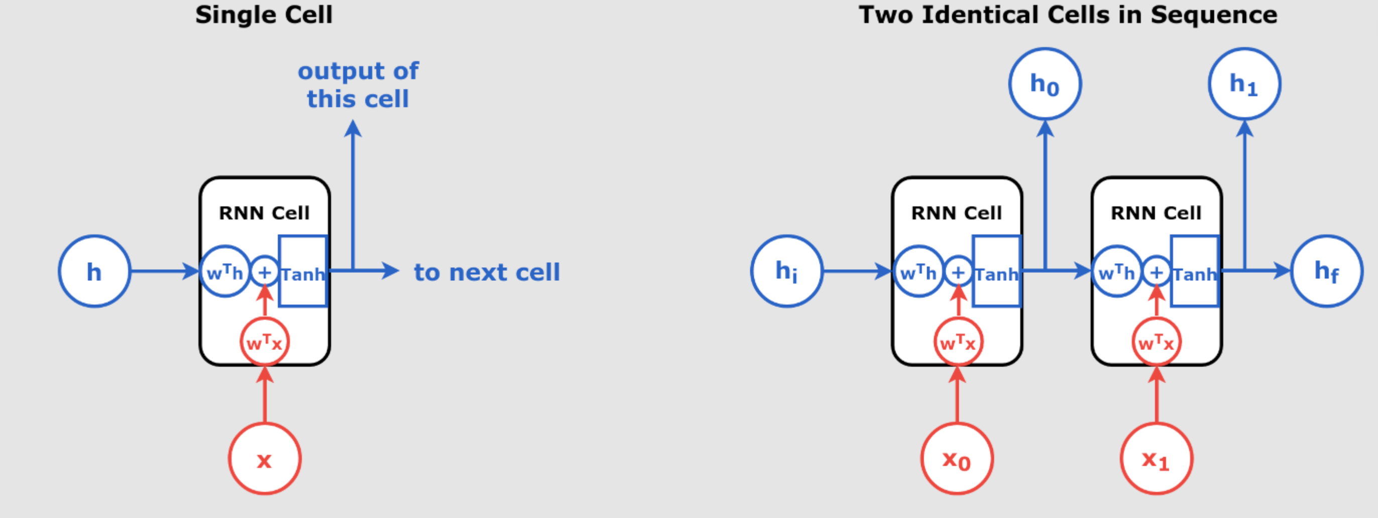
In iterative forecasting, the model predicts one time step ahead and uses that prediction as an input to predict the next step during inference.
Iteration 1
Forward Pass
We compute the hidden states and outputs for each time step.
Time Step  |  |  |  |  |  |
|---|---|---|---|---|---|
| 1 | 1 | 0 |  |  |  |
| 2 | 2 | 0.291 |  |  |  |
| 3 | 3 | 0.569 |  |  |  |
 depends on the previous hidden state and the current input , showcasing the sequential processing of RNNs.
Loss Calculation
Compute the Mean Squared Error (MSE):

| Time Step |  |  |  |
|---|---|---|---|
| 1 | 0.291 | 2 |  |
| 2 | 0.569 | 3 |  |
| 3 | 0.755 | 4 |  |
| Total | Sum = 19.337 | ||
| MSE |  | ||
Backpropagation
Step 1: Gradients w.r.t Outputs

| Time Step | | | |
|---|---|---|---|
| 1 | 0.291 | 2 |  |
| 2 | 0.569 | 3 |  |
| 3 | 0.755 | 4 |  |
Step 2: Gradients w.r.t and 


Compute:


Step 3: Gradients w.r.t Hidden States
Starting from the last time step and moving backward.
At  :
:

Compute:

 is used because of the tanh activation.
At  :
:

Compute:


At  :
:

Compute:


Step 4: Gradients w.r.t  ,
,  , and
, and 
Compute:


Calculations:
- For :

:

:

<
Mastering Time Series Forecasting with RNNs and Seq2Seq Models
Step 5: Update Weights and Biases
Update parameters using gradient descent:
\[ W_y^{\text{new}} = W_y – \eta \frac{\partial L}{\partial W_y} = 1.0 – 0.01 \times (-4.326) = 1.043 \]
\[ b_y^{\text{new}} = b_y – \eta \frac{\partial L}{\partial b_y} = 0.0 – 0.01 \times (-7.385) = 0.074 \]
\[ W_h^{\text{new}} = W_h – \eta \frac{\partial L}{\partial W_h} = 0.5 – 0.01 \times (-1.410) = 0.514 \]
\[ W_x^{\text{new}} = W_x – \eta \frac{\partial L}{\partial W_x} = 0.2 – 0.01 \times (-10.945) = 0.309 \]
\[ b_h^{\text{new}} = b_h – \eta \frac{\partial L}{\partial b_h} = 0.1 – 0.01 \times (-6.041) = 0.161 \]
Iteration 2
Using updated parameters.
Forward Pass
| Time Step | | |  | | |
|---|---|---|---|---|---|
| 1 | 1 | 0 |  |  |  |
| 2 | 2 | 0.438 |  |  |  |
| 3 | 3 | 0.759 |  |  |  |
Loss Calculation
| Time Step | | | |
|---|---|---|---|
| 1 | 0.530 | 2 |  |
| 2 | 0.866 | 3 |  |
| 3 | 1.019 | 4 |  |
| Total | Sum = 15.586 | ||
| MSE |  | ||
Backpropagation
Repeat the same backpropagation steps as in Iteration 1, using the updated parameters..
2. Direct Multi-Step Forecasting with RNN
In direct multi-step forecasting, the model predicts multiple future time steps simultaneously using the final hidden state of the RNN, without feeding predictions back into the model.
Iteration 1
Forward Pass
We process the input sequence to obtain the final hidden state and then predict multiple future outputs.
Time Step  |  |  |  |  |
|---|---|---|---|---|
| 1 | 1 | 0 |  |  |
| 2 | 2 | 0.291 |  |  |
| 3 | 3 | 0.569 |  |  |
 .
.Predict Outputs:
Assuming  is adjusted to output two values:
- Let be a
 matrix:

Compute the predictions:

Loss Calculation
Compute the Mean Squared Error (MSE):

Output Index  |  |  |  |
|---|---|---|---|
| 1 | 0.755 | 4 |  |
| 2 | 0.604 | 5 |  |
| Total | Sum = 29.839 | ||
| MSE |  | ||
Backpropagation
Step 1: Gradients w.r.t Outputs

Compute:


Step 2: Gradients w.r.t and 


is calculated using the final hidden state and the errors from both outputs.Step 3: Gradient w.r.t Final Hidden State

Compute derivative through the activation function:

Step 4: Backpropagate to Previous Time Steps
Compute  for
for  and
and  :
:
- At :

:

Step 5: Gradients w.r.t  ,
,  , and
, and 
Compute:
- For :

:

:

Step 6: Update Weights and Biases
Update parameters:


Iteration 2
Forward Pass
| Time Step | | |  |  |
|---|---|---|---|---|
| 1 | 1 | 0 |  |  |
| 2 | 2 | 0.425 |  |  |
| 3 | 3 | 0.765 |  |  |
Predict Outputs

Loss Calculation
| Output Index | | | |
|---|---|---|---|
| 1 | 1.000 | 4 |  |
| 2 | 0.807 | 5 |  |
| Total | Sum = 26.550 | ||
| MSE |  | ||
Backpropagation
Repeat the backpropagation steps as in Iteration 1, using updated parameters and calculations.
3. Seq2Seq Models for Time Series Forecasting
Seq2Seq models use an encoder-decoder architecture to handle input and output sequences of different lengths.
Iteration 1
Forward Pass
Encoder
Process input sequence ![X = [1, 2, 3]](https://ingoampt.com/wp-content/ql-cache/quicklatex.com-3b5f93a6a5673bb17412141350bd2cda_l3.png "Rendered by QuickLaTeX.com") to obtain the final hidden state
to obtain the final hidden state  .
.
| Encoder Time Step | | | | |
|---|---|---|---|---|
| 1 | 1 | 0 | | |
| 2 | 2 | 0.291 | | |
| 3 | 3 | 0.569 | | |
Decoder
Initialize decoder hidden state  . Assuming teacher forcing, we use the actual previous output as input.
- Decoder Weights: We’ll use separate weights for the decoder:


| Decoder Time Step |  | | | |  |
|---|---|---|---|---|---|
| 1 | 0 (start token) | 0.755 |  |  |  |
| 2 | 2 | 0.503 |  |  |  |
| 3 | 3 | 0.717 |  |  |  |
Loss Calculation
Compute the MSE over the decoder outputs:

| Time Step | |  |  |
|---|---|---|---|
| 1 | 0.503 | 2 |  |
| 2 | 0.717 | 3 |  |
| 3 | 0.837 | 4 |  |
| Total | Sum = 17.461 | ||
| MSE |  | ||
Backpropagation
Step 1: Gradients w.r.t Decoder Outputs

Compute:


Step 2: Backpropagation Through Decoder Time Steps
Compute gradients w.r.t decoder weights and biases.
At  :
:

At :


At :


Step 3: Gradients w.r.t Decoder Weights and Biases
Compute:
- For
 :
:


- Total:

 :
:


- Total:

 :
:


- Total:

 :
:

Step 4: Gradient w.r.t Encoder’s Final Hidden State
Since  , we need to compute:

Step 5: Backpropagation Through Encoder Time Steps
Compute for encoder time steps  :
:
- At :

:

:

Step 6: Gradients w.r.t Encoder Weights and Biases
Compute:
- For :

:

:

Iteration 2
Using updated parameters, repeat the forward pass and backpropagation steps for both the encoder and decoder.
By providing detailed calculations, tables, and highlighting method-specific features during the calculations, we’ve covered the 3 methods: Iterative Forecasting which is Predicting One Step at a Time and Direct Multi-Step Forecasting with RNN and Seq2Seq Models for Time Series Forecasting, demonstrating how each method processes data differently and how backpropagation is performed uniquely in each case.
Key Notes: Time Series Forecasting Methods Comparison
Here is a more detailed comparison of the three time series forecasting methods, including which is likely to have less error and insights into their current popularity based on 2024 trends.
Complete Table Comparing the Forecasting Methods
| Method | Prediction Style | When to Use | Drawbacks | Example Use Case | Error Propensity | Popularity in 2024 |
|---|---|---|---|---|---|---|
| Iterative Forecasting | Predicts one step at a time | When future depends on the immediate past (short-term) | Error accumulation due to feedback | Stock prices or energy consumption prediction | High error potential (due to error feedback) | Commonly used for simple tasks |
| Direct Multi-Step Forecasting | Predicts multiple steps at once | When future steps are loosely connected (medium-term) | May miss time step dependencies | Sales forecasting for the next few months | Moderate error, but no feedback loop errors | Moderate use, effective for medium-term |
| Seq2Seq Models | Encoder-decoder for full sequence | For long-term predictions or variable-length sequences | More complex and harder to train | Long-term financial forecasts or weather predictions | Lower error for complex or long-term tasks | Increasingly popular for complex forecasting, especially in deep learning |
Text-Based Graph Representations for Each Method
1. Iterative Forecasting (Predicting One Step at a Time)
This method predicts one step at a time and uses the predicted output as input for the next step, introducing a feedback loop.
Input:    [X₁, X₂, X₃]    --->   Y₁
                     |             |
                     v             v
Next Input: [X₂, X₃, Y₁] --->   Y₂
                     |             |
                     v             v
Next Input: [X₃, Y₁, Y₂] --->   Y₃
Error Propensity: As each prediction is used in the next step, errors from one prediction propagate through subsequent steps, leading to higher cumulative error.
2. Direct Multi-Step Forecasting with RNN
This method predicts multiple future steps at once, based on the input sequence, without any feedback loop.
Input: [X₁, X₂, X₃] ---> [Y₁, Y₂, Y₃]
Error Propensity: The model outputs multiple predictions at once, which can lead to moderate error, but avoids feedback loop problems.
3. Seq2Seq Models for Time Series Forecasting
Seq2Seq models use an encoder-decoder architecture, where the encoder processes the input sequence into a context vector, and the decoder generates the future sequence.
Encoder: [X₁, X₂, X₃] ---> Context Vector ---> Decoder: [Y₁, Y₂, Y₃]
Error Propensity: This model has lower error when applied to complex and long-term time series forecasting problems, as it captures dependencies across the entire sequence.
Still not clear ?
We know it sounds complicated at first ,
Therefore, Lets explain another way :
Part 1: Iterative Forecasting (One Step at a Time)
Training Process
The model predicts one time step ahead and feeds that prediction as input for the next step.
Example Input: [1, 2, 3] → Predicted Output (during training): [2, 3, 4]
Inference Process
During inference, the model predicts unseen future values based on new inputs.
Example Input: [3, 4, 5] → Predicted Output (during inference): [6, 7]
Loss Calculation
The model calculates the error between the predicted value and the actual target:

The total loss is summed over all predictions.
Backpropagation & Weight Updates
After each time step, the model uses Backpropagation Through Time (BPTT) to calculate the gradients and update the weights:

Where  is the learning rate, and
  is the gradient of the loss.
Graph Representation
Training:
Input: [1, 2, 3]    --->   Y₁ = 2
  Calculate Loss    --->   Update weights for Y₁
                     |
                     v
Next Input: [2, 3, Y₁] --->   Y₂ = 3
  Calculate Loss    --->   Update weights for Y₂
                     |
                     v
Next Input: [3, Y₁, Y₂] --->   Y₃ = 4
  Calculate Loss    --->   Update weights for Y₃
Inference:
Input: [3, 4, 5] ---> Model predicts Y₁ = 6, Y₂ = 7
Error Accumulation
Since each prediction depends on the previous step’s prediction, any errors from one prediction will propagate forward, leading to higher loss over time.
Pros
- Useful for short-term predictions where immediate dependencies exist between time steps.
Cons
- Error accumulation: If the early predictions are wrong, subsequent steps are affected, which increases the overall error.
Part 2: Direct Multi-Step Forecasting
Training Process
The model predicts multiple future values at once without feeding the predictions back into the input.
Example Input: [1, 2, 3] → Predicted Output: [4, 5]
Inference Process
In inference, the model predicts multiple future values based on the new unseen input.
Example Input: [3, 4, 5] → Predicted Output: [6, 7]
Loss Calculation
The loss is calculated simultaneously for all predictions:
Backpropagation & Weight Updates
The model adjusts its weights after all predictions are made:
Graph Representation
Training:
Input: [1, 2, 3]    --->   Y₁ = 4, Y₂ = 5
  Calculate Total Loss (for Y₁ and Y₂) --->   Update weights
Inference:
Input: [3, 4, 5] ---> Model predicts Y₁ = 6, Y₂ = 7
No Error Accumulation
Since all future steps are predicted at once, there is no error propagation between predictions, which can result in more accurate predictions.
Pros
- Suitable for medium-term forecasting tasks where multiple predictions are needed at once.
- Avoids the issue of feedback loops.
Cons
- It may miss some time dependencies between individual time steps, especially if they are strongly connected.
Part 3: Seq2Seq Models (Encoder-Decoder Architecture)
Training Process
The model uses an encoder-decoder structure, where the encoder processes the input sequence into a context vector, and the decoder generates the output sequence based on that vector.
Example Input: [1, 2, 3] → Predicted Output: [4, 5]
Inference Process
The model predicts unseen future values based on new inputs and the context vector generated by the encoder.
Example Input: [3, 4, 5] → Predicted Output: [6, 7]
Loss Calculation
The total loss is calculated across all predicted outputs:

Backpropagation & Weight Updates
The model uses Backpropagation Through Time (BPTT) to update the weights in both the encoder and decoder:


Graph Representation
Training:
Encoder: [1, 2, 3] ---> Context Vector
                                      |
                                      v
Decoder: Context Vector ---> Y₁ = 4, Y₂ = 5
  Calculate Total Loss ---> Update weights for encoder and decoder
Inference:
Encoder: [3, 4, 5] ---> Model predicts Y₁ = 6, Y₂ = 7
Long-Term Dependencies
The Seq2Seq architecture is highly effective at capturing long-term dependencies between input and output sequences. The context vector provides a summary of the entire input, allowing for more accurate predictions over longer time horizons.
Pros
- Best for long-term forecasting, especially when there are complex relationships between different time steps.
- The encoder-decoder structure is powerful in handling variable-length sequences.
Cons
- Requires more computational resources due to its complexity.
- May need more training data to perform well.
Final Thoughts: Choosing the Best Method
Each forecasting method has its strengths and weaknesses:
- Iterative Forecasting: Ideal for short-term predictions where there are immediate dependencies between the time steps, but it suffers from error accumulation, which can lead to higher overall loss over time.
- Direct Multi-Step Forecasting: This method avoids error feedback by predicting all future steps simultaneously, making it more suitable for medium-term forecasting. However, it might miss dependencies between individual time steps if the time steps are strongly connected.
- Seq2Seq Models: Best for long-term predictions where each future step depends on the entire input sequence. The encoder-decoder architecture is powerful for complex and variable-length sequences but requires more computational resources and data to achieve good performance.
Which Method Decreases Loss Better?
In summary, the method that decreases loss better depends on the forecasting task:
- Iterative Forecasting: Works well for short-term forecasting but suffers from error propagation.
- Direct Multi-Step Forecasting: Effective when you need to predict multiple steps at once without feedback loops. However, it may miss subtle time dependencies.
- Seq2Seq Models: Generally offer better performance in long-term forecasting because they capture complex dependencies across the entire input sequence. This helps reduce loss for complex tasks, but they require more training data and computational power.
Final Recommendation
Choosing the right forecasting method depends on the task at hand:
- If you are predicting short-term sequences with immediate dependencies, use Iterative Forecasting.
- If you need multiple steps predicted at once without worrying about feedback loops, opt for Direct Multi-Step Forecasting.
- If you’re working with long-term forecasts and complex relationships between inputs and outputs, the Seq2Seq Model will likely be the best choice.
Now is Time for Coding
Part 1: Iterative Forecasting (One Step at a Time)
Example:
- Input Sequence: [1, 2, 3]
- Target Sequence (during training): [4] (the next time step)
Explanation:
- One-Step Prediction:
- The model is trained to predict the next time step based on the input sequence.
- Iterative Inference:
- During inference (testing), the model uses its previous predictions as input to predict subsequent steps.
- Key Difference:
- The model outputs a single value at each step, making predictions iteratively for multi-step forecasting.
PyTorch Code Example
import torch
import torch.nn as nn
import torch.optim as optim

# Define the RNN model for Iterative Forecasting
class IterativeRNN(nn.Module):
    def __init__(self, input_size, hidden_size, output_size):
        super(IterativeRNN, self).__init__()
        self.rnn = nn.RNN(input_size, hidden_size, batch_first=True)
        self.fc = nn.Linear(hidden_size, output_size)  # Predicts one time step ahead

    def forward(self, x, hidden):
        # Pass input through RNN layer
        out, hidden = self.rnn(x, hidden)
        # Output only the last time step for prediction
        out = self.fc(out[:, -1, :])
        return out, hidden

# Hyperparameters
input_size = 1  # Feature dimension
hidden_size = 10  # Number of hidden units
output_size = 1  # Predicting one value
learning_rate = 0.01
num_epochs = 100

# Training data
x_train = torch.tensor([[[1.0], [2.0], [3.0]]])  # Shape: (batch_size, seq_length, input_size)
y_train = torch.tensor([[4.0]])  # Shape: (batch_size, output_size)

# Initialize the model, loss function, and optimizer
model = IterativeRNN(input_size, hidden_size, output_size)
criterion = nn.MSELoss()  # Mean Squared Error for regression tasks
optimizer = optim.Adam(model.parameters(), lr=learning_rate)

# Training loop
for epoch in range(num_epochs):
    model.train()
    optimizer.zero_grad()  # Reset gradients
    hidden = torch.zeros(1, x_train.size(0), hidden_size)  # Initialize hidden state
    output, hidden = model(x_train, hidden)  # Forward pass
    loss = criterion(output, y_train)  # Calculate loss
    loss.backward()  # Backpropagation
    optimizer.step()  # Update weights

    if (epoch + 1) % 10 == 0:
        print(f'Epoch [{epoch + 1}/{num_epochs}], Loss: {loss.item():.4f}')

# Inference: Predicting future values iteratively
model.eval()
with torch.no_grad():
    input_seq = x_train.clone()  # Start with the training input
    hidden = torch.zeros(1, input_seq.size(0), hidden_size)  # Initialize hidden state
    num_predictions = 2  # Number of future steps to predict
    predictions = []
    for _ in range(num_predictions):
        output, hidden = model(input_seq, hidden)  # Predict next step
        predictions.append(output.item())  # Save prediction
        # Update input sequence by appending the prediction
        input_seq = torch.cat((input_seq[:, 1:, :], output.unsqueeze(0).unsqueeze(2)), dim=1)
    print('Predicted values:', predictions)
Explanation
- Model Definition:
- Line 9:
self.fc = nn.Linear(hidden_size, output_size)
Explanation: The fully connected layer outputs a single time step ahead. - Line 13:
out = self.fc(out[:, -1, :])
Explanation: The model only uses the last time step’s hidden state to make a prediction.
- Line 9:
- Training Loop:
- Loss Function: The model uses Mean Squared Error (
nn.MSELoss) for regression tasks. - Gradient Update: Gradients are calculated and applied via backpropagation (
loss.backward()andoptimizer.step()).
- Loss Function: The model uses Mean Squared Error (
- Inference Loop:
- Line 45:
input_seq = torch.cat((input_seq[:, 1:, :], output.unsqueeze(0).unsqueeze(2)), dim=1)
Explanation: The previous input sequence is updated by dropping the oldest value and appending the new prediction, enabling iterative forecasting.
- Line 45:
—
Part 2: Direct Multi-Step Forecasting
Example:
- Input Sequence: [1, 2, 3]
- Target Sequence: [4, 5] (future values)
Explanation:
- Multi-Step Prediction:
- The model is trained to predict multiple future time steps simultaneously.
- Final Hidden State Usage:
- It uses the final hidden state to directly predict all future values without iterative feedback.
- Key Difference:
- The output layer predicts all future steps at once, rather than one step at a time.
PyTorch Code Example
import torch
import torch.nn as nn
import torch.optim as optim

# Define the RNN model for Direct Multi-Step Forecasting
class DirectMultiStepRNN(nn.Module):
    def __init__(self, input_size, hidden_size, output_size, num_future_steps):
        super(DirectMultiStepRNN, self).__init__()
        self.rnn = nn.RNN(input_size, hidden_size, batch_first=True)
        # Output layer predicts multiple future steps
        self.fc = nn.Linear(hidden_size, output_size * num_future_steps)
        self.num_future_steps = num_future_steps
        self.output_size = output_size

    def forward(self, x, hidden):
        # Pass input through RNN layer
        out, hidden = self.rnn(x, hidden)
        # Use the final hidden state to predict future steps
        out = self.fc(out[:, -1, :])  # Only the final time step
        # Reshape output to (batch_size, num_future_steps, output_size)
        out = out.view(-1, self.num_future_steps, self.output_size)
        return out, hidden


# Hyperparameters
input_size = 1  # Feature dimension
hidden_size = 10  # Number of hidden units
output_size = 1  # Predicting one feature per step
num_future_steps = 2  # Predicting two future steps
learning_rate = 0.01
num_epochs = 100

# Training data
x_train = torch.tensor([[[1.0], [2.0], [3.0]]])  # Shape: (batch_size, seq_length, input_size)
y_train = torch.tensor([[[4.0], [5.0]]])  # Shape: (batch_size, num_future_steps, output_size)

# Initialize the model, loss function, and optimizer
model = DirectMultiStepRNN(input_size, hidden_size, output_size, num_future_steps)
criterion = nn.MSELoss()  # Mean Squared Error for regression tasks
optimizer = optim.Adam(model.parameters(), lr=learning_rate)

# Training loop
for epoch in range(num_epochs):
    model.train()
    optimizer.zero_grad()  # Reset gradients
    hidden = torch.zeros(1, x_train.size(0), hidden_size)  # Initialize hidden state
    output, hidden = model(x_train, hidden)  # Forward pass
    loss = criterion(output, y_train)  # Calculate loss
    loss.backward()  # Backpropagation
    optimizer.step()  # Update weights

    if (epoch + 1) % 10 == 0:
        print(f'Epoch [{epoch + 1}/{num_epochs}], Loss: {loss.item():.4f}')

# Inference: Predicting future values
model.eval()
with torch.no_grad():
    input_seq = x_train.clone()  # Use the training input
    hidden = torch.zeros(1, input_seq.size(0), hidden_size)  # Initialize hidden state
    output, hidden = model(input_seq, hidden)  # Predict future steps
    predictions = output.squeeze().numpy()  # Convert predictions to numpy for readability
    print('Predicted values:', predictions)
Explanation:
- Model Definition:
- Line 10:
self.fc = nn.Linear(hidden_size, output_size * num_future_steps)
Explanation: This defines the fully connected layer, which outputs predictions for all future steps in one pass.
- Line 10:
- Forward Method:
- Line 16:
out = out.view(-1, self.num_future_steps, self.output_size)
Explanation: This reshapes the raw output from the fully connected layer into a format matching the target shape, i.e.,(batch_size, num_future_steps, output_size).
- Line 16:
- Training Loop:
- The training loop optimizes the model using Mean Squared Error loss (
nn.MSELoss), which is standard for regression tasks. - The hidden state is initialized and reset for each batch during training.
- The training loop optimizes the model using Mean Squared Error loss (
- Inference:
- The trained model directly predicts multiple future steps without using its predictions as inputs (no iterative feedback).
- The predictions are reshaped and returned for analysis.
—
Part 3: Seq2Seq Models (Encoder-Decoder Architecture)
Example:
- Input Sequence: [1, 2, 3]
- Target Sequence: [4, 5] (predicted output sequence)
Explanation:
- The model uses an encoder to process the input sequence into a context vector.
- A decoder generates the output sequence based on the context vector.
- Key Differences:
- Separate encoder and decoder networks.
- Use of teacher forcing during training.
PyTorch Code Example
import torch
import torch.nn as nn
import torch.optim as optim

# Define the Encoder
class EncoderRNN(nn.Module):
    def __init__(self, input_size, hidden_size):
        super(EncoderRNN, self).__init__()
        self.rnn = nn.RNN(input_size, hidden_size, batch_first=True)

    def forward(self, x, hidden):
        out, hidden = self.rnn(x, hidden)
        return hidden  # Return final hidden state

# Define the Decoder
class DecoderRNN(nn.Module):
    def __init__(self, hidden_size, output_size):
        super(DecoderRNN, self).__init__()
        self.rnn = nn.RNN(output_size, hidden_size, batch_first=True)
        self.fc = nn.Linear(hidden_size, output_size)

    def forward(self, x, hidden):
        out, hidden = self.rnn(x, hidden)
        out = self.fc(out)  # Apply output layer to each time step
        return out, hidden

# Hyperparameters
input_size = 1
hidden_size = 10
output_size = 1
learning_rate = 0.01
num_epochs = 100

# Training data
x_train = torch.tensor([[[1.0], [2.0], [3.0]]])  # Shape: (batch_size, seq_length, input_size)
y_train = torch.tensor([[[4.0], [5.0]]])  # Shape: (batch_size, target_length, output_size)

# Initialize models, loss function, and optimizers
encoder = EncoderRNN(input_size, hidden_size)
decoder = DecoderRNN(hidden_size, output_size)
criterion = nn.MSELoss()
encoder_optimizer = optim.Adam(encoder.parameters(), lr=learning_rate)
decoder_optimizer = optim.Adam(decoder.parameters(), lr=learning_rate)

# Training loop
for epoch in range(num_epochs):
    encoder.train()
    decoder.train()
    encoder_optimizer.zero_grad()
    decoder_optimizer.zero_grad()

    # Initialize hidden states
    encoder_hidden = torch.zeros(1, x_train.size(0), hidden_size)

    # Encoder forward pass
    encoder_hidden = encoder(x_train, encoder_hidden)  # Separate encoder

    # Decoder forward pass
    decoder_input = torch.zeros(x_train.size(0), 1, output_size)  # Start token
    decoder_hidden = encoder_hidden  # Decoder hidden state initialized with encoder hidden state
    target_length = y_train.size(1)
    outputs = torch.zeros(x_train.size(0), target_length, output_size)

    # Teacher forcing: use actual target outputs as next inputs
    for t in range(target_length):
        decoder_output, decoder_hidden = decoder(decoder_input, decoder_hidden)
        outputs[:, t:t+1, :] = decoder_output
        decoder_input = y_train[:, t:t+1, :]  # Teacher forcing applied

    # Compute loss
    loss = criterion(outputs, y_train)
    loss.backward()
    encoder_optimizer.step()
    decoder_optimizer.step()

    if (epoch + 1) % 10 == 0:
        print(f'Epoch [{epoch + 1}/{num_epochs}], Loss: {loss.item():.4f}')

# Inference: Predicting future values
encoder.eval()
decoder.eval()
with torch.no_grad():
    input_seq = x_train
    encoder_hidden = torch.zeros(1, input_seq.size(0), hidden_size)
    encoder_hidden = encoder(input_seq, encoder_hidden)

    decoder_input = torch.zeros(input_seq.size(0), 1, output_size)  # Start token
    decoder_hidden = encoder_hidden
    predictions = []
    target_length = 2  # Number of future steps to predict

    for _ in range(target_length):
        decoder_output, decoder_hidden = decoder(decoder_input, decoder_hidden)
        predictions.append(decoder_output.item())
        decoder_input = decoder_output  # Decoder uses its own output as next input

    print('Predicted values:', predictions)
Explanation:
- Separate Encoder and Decoder:
- Lines 7-17: Definition of
EncoderRNNandDecoderRNNclasses.
Explanation: These separate classes handle the encoding and decoding of sequences.
- Lines 7-17: Definition of
- Encoder Forward Pass:
- Line 43:
encoder_hidden = encoder(x_train, encoder_hidden)
Explanation: The encoder processes the input sequence into a context vector.
- Line 43:
- Decoder Initialization:
- Line 46:
decoder_hidden = encoder_hidden
Explanation: The decoder’s hidden state is initialized using the encoder’s final hidden state. This is the key difference in Seq2Seq models.
- Line 46:
- Teacher Forcing:
- Line 53:
decoder_input = y_train[:, t:t+1, :]
Explanation: During training, the actual target output is used as the next input to the decoder. This is called teacher forcing and helps the model learn faster.
- Line 53:
- Inference Without Teacher Forcing:
- Line 67:
decoder_input = decoder_output
Explanation: During inference, the decoder uses its own previous output as the next input.
- Line 67:
Summary of Key Differences
Iterative Forecasting:
- Output Layer Definition:
self.fc = nn.Linear(hidden_size, output_size) # Predicts one step ahead - Forward Method:
out = self.fc(out[:, -1, :]) # Only last output used - Inference Loop:
input_seq = torch.cat((input_seq[:, 1:, :], output.unsqueeze(0).unsqueeze(2)), dim=1) # Iterative feedback
Direct Multi-Step Forecasting:
- Output Layer Definition:
self.fc = nn.Linear(hidden_size, output_size * num_future_steps) # Predicts multiple steps - Forward Method:
out = self.fc(out[:, -1, :])       # Final hidden state used
out = out.view(-1, self.num_future_steps, self.output_size)  # Reshape for multiple steps
Seq2Seq Models:
- Separate Encoder and Decoder Classes:
class EncoderRNN(nn.Module): # Encoder definition class DecoderRNN(nn.Module): # Decoder definition - Decoder Initialization:
decoder_hidden = encoder_hidden # Decoder uses encoder's final hidden state - Teacher Forcing:
decoder_input = y_train[:, t:t+1, :] # Teacher forcing - Inference Without Teacher Forcing:
decoder_input = decoder_output # Decoder uses its own output
By comparing the lines of code across the three models, the specific features and techniques for each method become clear. Iterative forecasting uses feedback loops, direct multi-step forecasting predicts multiple steps simultaneously, and Seq2Seq models employ separate encoder and decoder networks with teacher forcing during training.