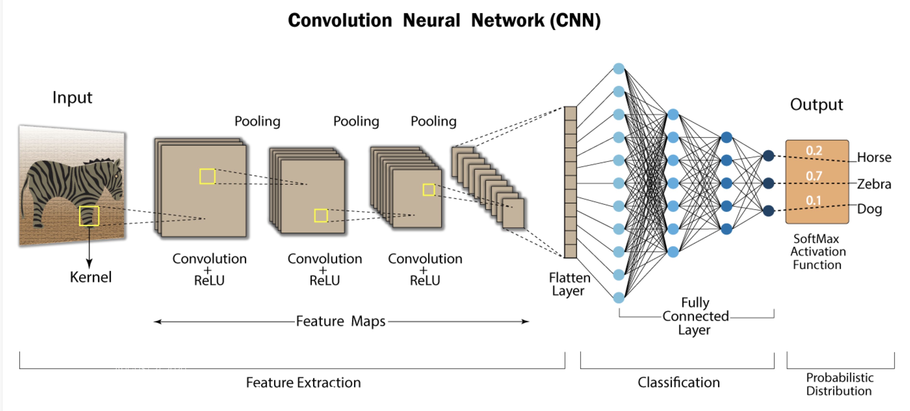
You have seen what CNNs are in our previous article.
Now, let’s explore the mathematics behind CNNs in detail, step by step, with a very simple example.
Part 1: Input Layer, Convolution, and Pooling (Steps 1-4)
Step 1: Input Layer
We are processing two 3×3 grayscale images—one representing a zebra and one representing a cat.
Image 1: Zebra Image (e.g., with stripe-like patterns)

Image 2: Cat Image (e.g., with smoother, fur-like textures)

These images are represented as 2D grids of pixel values, with each value between 0 and 1 indicating pixel intensity.
Step 2: Convolutional Layer (Feature Extraction)
We’ll apply a 3×3 convolutional filter to detect patterns such as edges. For simplicity, we’ll use the same filter for both images.
Convolution Filter (Edge Detector):

Convolution on the Zebra Image
For the first patch (the full 3×3 grid), the element-wise multiplication with the filter is:


Summing the values:

The feature map value for this part of the zebra image is 0.7.
Convolution on the Cat Image
Now, let’s perform the convolution on the cat image.


Summing the values:

The feature map value for this part of the cat image is -0.3.
Step 3: ReLU Activation (Non-Linearity)
The ReLU activation function converts all negative values to 0 while keeping positive values unchanged.
- Zebra Image (after ReLU):
 remains 0.7.
 - Cat Image (after ReLU):
 becomes 0.0.
Step 4: Pooling Layer (Downsampling)
Next, we apply max pooling to downsample the feature maps. For simplicity, let’s assume we reduce each feature map to a single value:
- Zebra Image (after pooling):
- Cat Image (after pooling):

Part 2: Fully Connected Layer (Step 5)
Now, we move to the fully connected layer, where we combine the features extracted from the convolutional layer and use weights and biases to compute the logits for each class.
Step 5: Fully Connected Layer – Weight and Bias Calculation
At this point, we’ve flattened the pooled outputs:
- Zebra Image (flattened):
![[0.7]](https://ingoampt.com/wp-content/ql-cache/quicklatex.com-50d971a9f19d2df86fe225afef8f2f3d_l3.png "Rendered by QuickLaTeX.com")
- Cat Image (flattened):
![[0.0]](https://ingoampt.com/wp-content/ql-cache/quicklatex.com-f3b668ac9ee22e95c0b0447049a446b5_l3.png "Rendered by QuickLaTeX.com")
The fully connected layer computes the logits for each class (zebra, cat) using weights and biases. For this step, we’ll show how weights and biases are applied, and how they are updated based on loss.
The formula for the logit of class  is:
is:

Where:
 is the weight for class ,
 is the feature value from the previous layer (e.g., ),
 is the bias for class ,
 is the logit for class (before applying Softmax).
Let’s assume the following initial weights and biases for each class:
- Zebra class: Initial weight:
 , Initial bias:
- Cat class: Initial weight:
 , Initial bias:
Logit Calculation for Zebra Image (Flattened Input: [0.7])
For the zebra class:

For the cat class:

Logit Calculation for Cat Image (Flattened Input: [0.0])
For the zebra class:

For the cat class:

Part 3: Loss Calculation and Weight/Bias Update (Backpropagation)
Now that we’ve computed the logits, we need to calculate the loss and perform backpropagation to update the weights and biases.
Loss Calculation (Cross-Entropy Loss)
We use cross-entropy loss to measure the difference between the predicted probabilities and the true labels. For simplicity, assume the true label for the zebra image is zebra (1), and the true label for the cat image is cat (1).
Cross-entropy loss formula for a single class:

Where:
 is the true label (1 for the correct class, 0 for the others),
 is the predicted probability for class .
First, we apply the Softmax function to convert the logits into probabilities.
Softmax for the Zebra Image:

- Zebra logit:

- Cat logit:

Exponentials:

Sum of exponentials:

Probabilities:
- Zebra:

- Cat:

Cross-Entropy Loss for Zebra Image:
Let’s assume the true label is “zebra” (1 for zebra, 0 for cat):
![\text{Loss}_{\text{zebra}} = -[1 \times \log(0.78) + 0 \times \log(0.22)] = -\log(0.78) \approx 0.249](https://ingoampt.com/wp-content/ql-cache/quicklatex.com-f112452d541eeb2a9dbebb77f8b358e0_l3.png "Rendered by QuickLaTeX.com")
This is the loss value for the zebra image.
Part 4: Weight and Bias Update Using Gradient Descent
Using the loss value, the network performs backpropagation to calculate the gradients (partial derivatives of the loss with respect to each weight and bias). These gradients are used to update the weights and biases to reduce the loss in the next iteration.
For simplicity, assume the gradients calculated for each weight and bias are as follows (based on chain rule and backpropagation):
- Gradient for zebra weight:

- Gradient for zebra bias:

- Gradient for cat weight:

- Gradient for cat bias:

Updated Weights and Biases
Using gradient descent, we update the weights and biases:

Where  is the learning rate (assume
  ):
):


For the cat class:


Recap
- The network computes logits using weights and biases.
- Softmax converts logits into probabilities.
- Cross-entropy loss measures the error, and gradients are computed through backpropagation.
- Gradients update the weights and biases to reduce the loss for the next iteration.
This entire process repeats until the network minimizes the loss and correctly classifies images of zebras and cats.
Part 5: Continuing the Process for Subsequent Iterations
Now that we’ve seen how the fully connected layer works and how weights and biases are updated in one iteration, let’s continue to show what happens in the following iterations as the network learns. The goal is to keep refining the weights and biases through backpropagation and gradient descent, so the network gets better at predicting whether the input is a zebra or a cat.
Updated Weights and Biases After First Iteration:
- Zebra class: Updated weight:
 , Updated bias:
- Cat class: Updated weight:
 , Updated bias:
Step 5: Fully Connected Layer Calculations for the Second Iteration
Logit Calculation for Zebra Image (Flattened Input: [0.7])
Now, using the updated weights and biases, we recalculate the logits for the zebra image.
For the zebra class:

For the cat class:

Logit Calculation for Cat Image (Flattened Input: [0.0])
For the zebra class:

For the cat class:

Step 6: Reapplying Softmax Function
Now, let’s apply the Softmax function to the updated logits to get the new predicted probabilities.
For the Zebra Image:
Logits:
- Zebra logit:

- Cat logit:

Exponentials:

Sum of exponentials:

Probabilities:
- Zebra:

- Cat:

For the Cat Image:
Logits:
- Zebra logit:

- Cat logit:

Exponentials:

Sum of exponentials:

Probabilities:
- Zebra:

- Cat:

Step 7: Recalculating Loss
Next, we calculate the cross-entropy loss for both images based on the updated predictions.
Loss for Zebra Image:
Assume the true label is still “zebra” (1 for zebra, 0 for cat). The cross-entropy loss is:
![\text{Loss}_{\text{zebra}} = -[1 \times \log(0.779) + 0 \times \log(0.221)] = -\log(0.779) \approx 0.249](https://ingoampt.com/wp-content/ql-cache/quicklatex.com-e20066925d755357819b4b5b2238e32b_l3.png "Rendered by QuickLaTeX.com")
Loss for Cat Image:
Assume the true label is still “cat” (0 for zebra, 1 for cat). The cross-entropy loss is:
![\text{Loss}_{\text{cat}} = -[0 \times \log(0.55) + 1 \times \log(0.45)] = -\log(0.45) \approx 0.799](https://ingoampt.com/wp-content/ql-cache/quicklatex.com-382069c2e3b3fe960d70b5f9b95c8533_l3.png "Rendered by QuickLaTeX.com")
Step 8: Further Weight and Bias Updates Using Backpropagation
Now, the network uses backpropagation to compute the gradients again and updates the weights and biases based on the new loss values. For simplicity, assume the gradients for this iteration are as follows:
- Gradient for zebra weight:

- Gradient for zebra bias:

- Gradient for cat weight:

- Gradient for cat bias:

Using gradient descent, the weights and biases are updated again:


Similarly, for the cat class:


Repeat the Process
This process of calculating logits, applying Softmax, calculating loss, and updating weights and biases continues over many iterations until the network minimizes the loss and correctly classifies images with high confidence. Over time, the network improves at distinguishing between zebra and cat features.
- Input: We started with two images (a zebra and a cat) as input to the CNN.
- Convolutional Layers: We applied a convolutional filter to detect edge features.
- ReLU: We applied the ReLU activation function to retain positive feature values.
- Pooling: We downsampled the feature map using max pooling.
- Fully Connected Layer: The flattened pooled values were multiplied by weights and added to biases to calculate logits.
- Softmax: We converted logits into probabilities using the Softmax function.
- Loss Calculation: We used cross-entropy loss to measure the error between the predicted and true labels.
- Backpropagation: Gradients were computed, and weights and biases were updated using gradient descent to minimize the loss.
- Iteration: This process repeated, with weights and biases gradually adjusting to improve classification performance.
This detailed process explains how the CNN learns over time to classify images like zebra and cat by adjusting weights and biases based on the loss function!
Part 6: Continuing with Next Iteration (Iteration 3)
At this point, we’ve already updated the weights and biases after two iterations. Let’s update them again and show how the network refines its predictions as we explained through the repeating the process .
Lets show the Updated Weights and Biases After Iteration 2
- Zebra class: Updated weight:
 , Updated bias:
- Cat class: Updated weight:
 , Updated bias:
Step 5: Fully Connected Layer Calculations for the Next Iteration
Logit Calculation for Zebra Image (Flattened Input: [0.7])
For the zebra class:

For the cat class:

Logit Calculation for Cat Image (Flattened Input: [0.0])
For the zebra class:

For the cat class:

Step 6: Softmax Calculation (Converting Logits to Probabilities)
Next, we apply the Softmax function to convert the logits into probabilities, which will tell us how confident the network is about the image being a zebra or a cat.
For the Zebra Image:
Logits:
- Zebra:

- Cat:

Exponentials:

Sum of exponentials:

Probabilities:
- Zebra:

- Cat:

For the Cat Image:
Logits:
- Zebra:

- Cat:

Exponentials:

Sum of exponentials:

Probabilities:
- Zebra:

- Cat:

Step 7: Final Classification Decision
At this point, we have the final probabilities for both the zebra and cat images.
- For the Zebra Image: The network is 78% confident that the image is a zebra and 22% confident that it’s a cat. Since the probability for zebra is higher, the network classifies the zebra image as a zebra.
- For the Cat Image: The network is 55% confident that the image is a zebra and 45% confident that it’s a cat. This is a borderline case, but the network leans slightly toward classifying the cat image as a zebra, though with low confidence.
Step 8: Improving the Network (More Iterations)
At this point, the network still isn’t confident enough about the cat image—the probability for zebra is still higher than for cat. However, the network will continue to update its weights and biases through more iterations to become better at identifying cat-specific features (like smooth textures or fur-like patterns) and distinguishing them from zebra-specific features (like stripes and edges).
After many more training iterations, the network will gradually improve its performance and reach higher confidence for classifying both zebras and cats. Over time, the probability for cat in the cat image will rise as the network learns to associate specific patterns with the correct class.
Notes
- The network processes each image through convolutional layers, ReLU, and pooling to extract features.
- In the fully connected layer, the network uses weights and biases to calculate logits for each class.
- The Softmax function converts these logits into probabilities, giving the network’s confidence in its predictions.
- After several iterations of training and weight updates, the network becomes confident that the zebra image is a zebra (with a 78% probability).
- The network is still unsure about the cat image but leans toward classifying it as a zebra (with 55% probability) due to insufficient training iterations.
By continuing the training process (more iterations), the network will eventually be able to classify both images with high confidence, reducing the classification error over time.
How the CNN Refines Its Predictions
This is how the CNN refines its predictions through the iterative process of backpropagation, weight updates, and loss minimization. With more training and weight adjustment, the network will improve and reduce the classification error for future inputs.
As a Perfect Example for CNN integration Check the INGOAMPT app called :background img remove INGOAMPT & Discover how the Ingoampt app leverages CNN deep learning through Apple’s Core ML technology. This is simple app is perfect example of using CNN as a service.
Wanna support INGOAMPT? Purchase our Apps to contribute & be part of our journey. Also you can email us at email@ingoampt.com
Click Here to Check Our app called Background Remove Image INGOAMPT as a perfect example of CNN & what we explained.
.
To Understand Deeper, Let’s See Another Example for Math Explanation. with Real Numbers :
Lets demystify CNNs by walking through a detailed example using for four simple images this time. We’ll explain each step thoroughly and delve into how the network processes images, makes predictions, and learns over time.
The Four-Image Example
To make CNNs more accessible, we’ll use a simplified example involving four images and two classes.
Classes and Images
Classes:
- Class 0: Cat
- Class 1: Dog
Images:
We have four 4×4 grayscale images, each represented as a matrix with pixel values of 0 or 1 for simplicity.
Image 1 (Cat):
[0, 1, 0, 1]
[0, 1, 0, 1]
[0, 1, 0, 1]
[0, 1, 0, 1]
Image 2 (Cat):
[1, 1, 1, 1]
[0, 0, 0, 0]
[1, 1, 1, 1]
[0, 0, 0, 0]
Image 3 (Dog):
[1, 0, 1, 0]
[0, 1, 0, 1]
[1, 0, 1, 0]
[0, 1, 0, 1]
Image 4 (Dog):
[1, 0, 0, 0]
[0, 1, 0, 0]
[0, 0, 1, 0]
[0, 0, 0, 1]
Simplified CNN Architecture
Our CNN will consist of the following layers and components:
- Convolutional Layer:
- Filters: 2 filters (Filter A and Filter B)
- Activation Function:
- ReLU (Rectified Linear Unit)
- Flattening: Convert feature maps into a feature vector
- Fully Connected Layer: Output layer with weights and biases
- Softmax Function: Convert logits into probabilities
- Loss Function: Cross-entropy loss
- Training Process: We’ll perform one iteration to demonstrate learning
Step-by-Step Processing of the Images
We’ll go through each step in detail, explaining how the CNN processes the images, makes predictions, and learns.
Step 1: Input Images
Let’s define our four images (as shown above).
Step 2: Defining the Filters
Filters (or kernels) are essential in CNNs for feature detection.
Filter A (Vertical Edge Detector):
[1, -1]
[1, -1]
This filter is designed to detect vertical edges by highlighting differences between adjacent columns.
Filter B (Horizontal Edge Detector):
[1, 1]
[-1, -1]
This filter detects horizontal edges by emphasizing differences between adjacent rows.
Step 3: Convolution Operation
We apply each filter to each image to produce feature maps.
Convolution Process:
- Sliding the Filter: The filter moves across the image, one pixel at a time.
- Element-wise Multiplication: At each position, the filter’s values are multiplied with the corresponding pixel values in the image.
- Summation: The results are summed to produce a single value for that position in the feature map.
Example: Convolution of Image 1 with Filter A
Let’s compute the convolution at position (0,0):
Region of Image:
[0, 1]
[0, 1]
Convolution Calculation:

We repeat this process for each valid position where the filter fits within the image. The results are compiled into a feature map.
Convolution Results for Image 1 with Filter A:
| Position | Region Covered | Convolution Result |
|---|---|---|
| (0,0) | [0,1],[0,1] | -2 |
| (0,1) | [1,0],[1,0] | 2 |
| (0,2) | [0,1],[0,1] | -2 |
| (1,0) | [0,1],[0,1] | -2 |
| (1,1) | [1,0],[1,0] | 2 |
| (1,2) | [0,1],[0,1] | -2 |
| (2,0) | [0,1],[0,1] | -2 |
| (2,1) | [1,0],[1,0] | 2 |
| (2,2) | [0,1],[0,1] | -2 |
Step 4: Activation Function
We apply the ReLU activation function to the convolution results. ReLU (Rectified Linear Unit) sets all negative values to zero, introducing non-linearity into the model.
Activated Feature Map for Image 1 with Filter A:
[0, 2, 0]
[0, 2, 0]
[0, 2, 0]
Explanation:
- Negative values become 0.
- Positive values remain unchanged.
We repeat the convolution and activation steps for each filter and each image.
Step 5: Flattening the Feature Maps
For each image, we flatten the activated feature maps into a single feature vector. This vector represents the presence and strength of features detected by the filters.
Feature Vector for Image 1:
- Flattened Feature Map from Filter A:
[0, 2, 0, 0, 2, 0, 0, 2, 0]
- Flattened Feature Map from Filter B:
[0, 0, 0, 0, 0, 0, 0, 0, 0]
- Combined Feature Vector (Length 18):
[0, 2, 0, 0, 2, 0, 0, 2, 0, 0, 0, 0, 0, 0, 0, 0, 0, 0]
Note:
- The first 9 elements correspond to Filter A.
- The next 9 elements correspond to Filter B.
Step 6: Fully Connected Layer
The fully connected layer combines the features extracted to make a prediction.
Weights and Biases:
- Weights for Cat (Class 0): A vector
 of length 18.
 - Weights for Dog (Class 1): A vector
 of length 18.
 - Biases:


Initialization: For simplicity, we initialize all weights as follows:
![w_{\text{cat}} = [0.1, 0.1, ..., 0.1]](https://ingoampt.com/wp-content/ql-cache/quicklatex.com-bc8657f86fe64482b76f5bede903b600_l3.png "Rendered by QuickLaTeX.com") (18 times)
(18 times)![w_{\text{dog}} = [0.05, 0.05, ..., 0.05]](https://ingoampt.com/wp-content/ql-cache/quicklatex.com-4168a566d856096fc5bbd26560648a24_l3.png "Rendered by QuickLaTeX.com") (18 times)
(18 times)
Step 7: Calculating Logits
We calculate the logits for each class by performing a weighted sum of the feature vector and adding the bias.
Formula:

Calculations for Image 1:
- Feature Vector
 :
:[0, 2, 0, 0, 2, 0, 0, 2, 0, 0, 0, 0, 0, 0, 0, 0, 0, 0]
- Logit for Cat (Class 0):


Step 8: Applying the Softmax Function
The Softmax function converts logits into probabilities, ensuring that they are positive and sum to 1.
Softmax Formula:

Calculations for Image 1:
- Exponentiate the logits:
- Sum of exponentials:


- Probability for Cat:


Step 9: Comparing Predicted Probabilities with True Labels
Now, we compare the network’s predictions with the true labels provided by humans.
- True Label for Image 1 (Cat):
[1, 0]
- Predicted Probabilities:
[0.786, 0.214]
Why Are They Comparable?
Understanding the Comparison:
- True Labels:
- Represented using one-hot encoding.
- For a cat image:
![[1, 0]](https://ingoampt.com/wp-content/ql-cache/quicklatex.com-6c12e8d7a03ae1b44d76ec46bfa53da8_l3.png "Rendered by QuickLaTeX.com") (100% cat, 0% dog).
(100% cat, 0% dog). - It’s a probability distribution where one class has a probability of 1, and the rest have 0.
- Predicted Probabilities:
- The network’s output after applying Softmax.
- For Image 1:
![[0.786, 0.214]](https://ingoampt.com/wp-content/ql-cache/quicklatex.com-d285c528ca6aa6ed1cedb6c9a69dde0b_l3.png "Rendered by QuickLaTeX.com") .
. - Represents the network’s confidence in each class.
Why They Are Comparable:
- Same Format:
- Both are vectors of the same length (number of classes).
- Each element corresponds to the same class in both vectors.
- Probability Distributions:
- Both represent probability distributions over the classes.
- True labels are the ground truth distributions.
- Predicted probabilities are the model’s estimated distributions.
Purpose of Comparison:
- Calculate Loss:
- By comparing these distributions, we can measure how well the model’s predictions match the true labels.
- Guide Learning:
- The discrepancy guides the adjustment of the network’s weights during training.
Mathematical Basis:
- Cross-Entropy Loss:
- Measures the difference between two probability distributions.
Conclusion:
The comparison is meaningful because it assesses how close the model’s predictions are to the true labels, enabling the network to learn from its mistakes.
Step 10: Calculating Loss
We use the cross-entropy loss function to quantify the error between the predicted probabilities and the true labels.
Cross-Entropy Loss Formula:

Calculations for Image 1:
- Given:
- Loss Calculation:


![\text{Loss} = -[1 \times \log(0.786) + 0 \times \log(0.214)] = -\log(0.786) \approx 0.241](https://ingoampt.com/wp-content/ql-cache/quicklatex.com-b5783c8403c39182d4d86a9b54211f2d_l3.png "Rendered by QuickLaTeX.com")
Explanation:
- The loss is higher when the predicted probability for the true class is lower.
- The loss function penalizes incorrect or uncertain predictions.
Step 11: Backpropagation and Weight Update
We update the network’s weights to minimize the loss using gradient descent.
Calculating Gradients:
- Error Signal for Each Class:


Updating Weights and Biases:
- Learning Rate (
 ): We use
  .
. - Update Rule for Weights:


Example Calculation for Cat Class:
- Updating a Single Weight (e.g.,
 ):
):

Substituting values:


Explanation:
- Weights Associated with Features Present in the Image:
- Since
 is negative, the weights for the “cat” class are increased (subtracting a negative value).
- Since
- Purpose of Weight Update:
- To increase the network’s confidence in predicting “cat” when these features are present.
Repeating for Dog Class:
Similar calculations are performed for the “dog” class weights and biases.
Understanding the Learning Process
By processing each image and updating the weights accordingly, the CNN learns to improve its predictions over time.
Key Points:
- Individual Image Processing:
- Each image is processed separately, and the network updates its weights based on the error for that specific image.
- Role of Filters:
- Filters detect features important for classification.
- During training, filters adjust to become more sensitive to features that help distinguish between classes.
- Comparison of Predicted Probabilities and True Labels:
- Essential for calculating the loss.
- Provides the feedback needed for the network to learn.
- Weight Updates:
- Weights are adjusted in the direction that minimizes the loss.
- Enhances the network’s ability to predict the correct class when specific features are present.
- Why the Values Are Comparable:
- Both the predicted probabilities and true labels are probability distributions over the same set of classes.
- Loss functions like cross-entropy are designed to compare such distributions effectively.
Outcome:
Over multiple iterations, the network becomes better at recognizing patterns associated with each class, leading to improved accuracy.
Conclusion
Now, Through this detailed example with 4 images, we’ve explored how a CNN processes images, makes predictions, and learns from its mistakes. By understanding each step in this example, we can appreciate how CNNs:
- Extract Features: Using filters to detect important patterns.
- Make Predictions: Combining features to compute probabilities.
- Learn and Improve: Adjusting weights based on the loss to enhance performance.
Final Thoughts:
The comparison between predicted probabilities and true labels is crucial because it quantifies how well the network is performing. This comparison drives the learning process, enabling the network to adjust its parameters and improve over time.
Understanding these concepts is fundamental to working with CNNs and applying them to real-world problems in computer vision.
About the Author
INGOAMPT is passionate about machine learning & Deep Learning. We aims to make complex concepts accessible to everyone. Do not Forget to check our iOS Apps which many of them integrate Machine Learning. Also, all articles available at our app of : AI ACADEMY : DEEP LEARNING APP
Do Not Forget To Stay Connected Because Much More Are Coming From INGOAMPT.
Feel free to email us for any questions regards our apps or tutorials and services at email@ingoampt.com