First check automatic – keras tuner – which is explained in our previous post Automated Hyperparameter Tuning in Keras Part 1: Automated Approaches for Hyperparameter Tuning in Keras Hyperparameter tuning is a crucial step in machine learning that involves finding the best set of parameters for your model to optimize its performance. Keras provides a robust toolset for this purpose through its KerasTuner library, which offers several powerful, automated methods to explore the hyperparameter space. In this section, we’ll dive into the different models and approaches available in Keras for automated hyperparameter tuning, updated with the latest in 2024. 1. Random Search Random search is one of the simplest and most straightforward hyperparameter tuning methods. It works by randomly sampling hyperparameter combinations from the predefined search space. Despite its simplicity, random search can be surprisingly effective, especially when combined with a well-chosen search space. It’s often used as a baseline method due to its ease of implementation and ability to explore diverse regions of the hyperparameter space. tuner = kt.RandomSearch( build_model, objective='val_accuracy', max_trials=10, executions_per_trial=2, directory='random_search_dir', project_name='random_search' ) tuner.search(x_train, y_train, epochs=5, validation_data=(x_val, y_val)) Here, max_trials defines the number of different hyperparameter combinations to try, while executions_per_trial allows for multiple runs to average out random variations. 2. Bayesian Optimization Bayesian Optimization is a more sophisticated approach that models the objective function to predict which hyperparameters might perform well, based on the results of previous trials. This method balances exploration of new areas of the hyperparameter space with exploitation of known good areas, making it more efficient than random search. tuner = kt.BayesianOptimization( build_model, objective='val_loss', max_trials=10, directory='bayesian_optimization_dir', project_name='bayesian_optimization' ) tuner.search(x_train, y_train, epochs=10, validation_data=(x_val, y_val)) This method is particularly useful when the search space is large or when computational resources are limited, as it tends to converge to good solutions faster than random search. 3. Hyperband Hyperband is a method designed to optimize the resource allocation for hyperparameter tuning. It starts by evaluating many configurations with a small budget (e.g., a few epochs) and progressively allocates more resources (e.g., more epochs) to the most promising configurations. This makes Hyperband particularly effective when training is expensive, as it avoids wasting resources on poor configurations. tuner = kt.Hyperband( build_model, objective='val_accuracy', max_epochs=20, factor=3, directory='hyperband_dir', project_name='hyperband' ) tuner.search(x_train, y_train, epochs=5, validation_data=(x_val, y_val)) Hyperband is known for its ability to efficiently handle large hyperparameter spaces by dynamically allocating resources based on performance. 4. Sklearn Tuner For users integrating Scikit-learn models with Keras, the Sklearn tuner allows hyperparameter tuning within the familiar KerasTuner framework. This tuner is especially useful when you have a hybrid workflow that involves both Scikit-learn and Keras models. tuner = kt.SklearnTuner( model_builder, objective='accuracy', max_trials=10, directory='sklearn_tuner_dir', project_name='sklearn_tuner' ) tuner.search(x_train, y_train, validation_data=(x_val, y_val)) This tuner provides flexibility in tuning a wide range of models beyond just those built with Keras. 5. Gemma Models with LoRA API (2024 Update) One of the latest advancements in 2024 is the introduction of Gemma models, a family of lightweight large language models (LLMs) that can be fine-tuned with Keras using the new LoRA (Low Rank Adaptation) API. This API enables parameter-efficient fine-tuning by drastically reducing the number of trainable parameters without compromising performance. gemma_lm = keras_nlp.models.GemmaCausalLM.from_preset("gemma_2b_en") gemma_lm.backbone.enable_lora(rank=4) gemma_lm.generate("Keras is a", max_length=32) This approach is ideal for deploying large models on resource-constrained environments like mobile devices or for applications where rapid fine-tuning is essential. Conclusion Automated hyperparameter tuning in Keras has evolved significantly, offering tools that range from simple random search methods to complex Bayesian optimization and cutting-edge approaches like the LoRA API for fine-tuning large language models. These tools empower developers to efficiently explore the hyperparameter space and build optimized models with minimal manual intervention. As next, Let’s check the Manual Tuning : Manual Hyperparameter Tuning in Keras Part 2: Manual Hyperparameter Tuning Strategies While automated hyperparameter tuning in Keras offers powerful and efficient ways to optimize models, there are situations where manual tuning can be invaluable. This approach allows for a deep understanding of how different parameters affect the model and can be particularly useful when dealing with smaller datasets, specific constraints, or when you need fine-grained control over the model’s performance. 1. Manual Grid Search Explanation Grid search involves creating a ‘grid’ of hyperparameter values and exhaustively testing every possible combination. It is a systematic and thorough approach, which guarantees finding the best combination within the predefined grid. However, it can be computationally expensive, especially when the grid is large. Example Let’s say we’re tuning an SVM model. We want to test specific values of C and gamma based on our prior knowledge. Manual Code Example from sklearn import datasets from sklearn.model_selection import train_test_split from sklearn.svm import SVC from sklearn.metrics import accuracy_score # Load a dataset X, y = datasets.load_iris(return_X_y=True) X_train, X_test, y_train, y_test = train_test_split(X, y, test_size=0.3, random_state=42) # Define manually selected parameters C_values = [0.1, 1, 10] gamma_values = [0.01, 0.1] best_score = 0 best_params = {} # Manual grid search for C in C_values: for gamma in gamma_values: # Train the model with selected hyperparameters svm = SVC(C=C, gamma=gamma) svm.fit(X_train, y_train) y_pred = svm.predict(X_test) # Evaluate the model score = accuracy_score(y_test, y_pred) print(f"C: {C}, Gamma: {gamma}, Accuracy: {score}") # Update the best parameters if current score is higher if score > best_score: best_score = score best_params = {'C': C, 'gamma': gamma} print(f'Best Score: {best_score}') print(f'Best Parameters: {best_params}') Resource: For more on Grid Search, see Analytics Vidhya’s guide. 2. Sequential Tuning Explanation Sequential tuning involves tuning one hyperparameter at a time. This approach allows you to see the impact of each hyperparameter independently before moving on to the next. Example For a neural network, start by finding the optimal learning rate, then adjust the number of neurons in the hidden layers. Manual Code Example from tensorflow.keras.models import Sequential from tensorflow.keras.layers import Dense from tensorflow.keras.optimizers import Adam from tensorflow.keras.datasets import mnist from tensorflow.keras.utils import to_categorical # Load the MNIST dataset (X_train, y_train), (X_test, y_test) = mnist.load_data() X_train, X_test = X_train.reshape(-1, 784), X_test.reshape(-1, 784) y_train, y_test = to_categorical(y_train), to_categorical(y_test) # Define a simple neural network model def build_model(learning_rate, neurons): model = Sequential([ Dense(neurons, input_shape=(784,), activation='relu'), Dense(10, activation='softmax') ]) model.compile(optimizer=Adam(learning_rate=learning_rate), loss='categorical_crossentropy', metrics=['accuracy']) return model # Step 1: Tune learning rate learning_rates = [0.01, 0.001, 0.0001] best_score = 0 best_lr = None for lr in learning_rates: model = build_model(lr, neurons=64) model.fit(X_train, y_train, epochs=5, batch_size=128, verbose=0) score = model.evaluate(X_test, y_test, verbose=0)[1] print(f"Learning Rate: {lr}, Accuracy: {score}") if score > best_score: best_score = score best_lr = lr print(f'Best Learning Rate: {best_lr}') # Step 2: Tune number of neurons using the best learning rate neuron_options = [32, 64, 128] best_neurons = None for neurons in neuron_options: model = build_model(best_lr, neurons=neurons) model.fit(X_train, y_train, epochs=5, batch_size=128, verbose=0) score = model.evaluate(X_test, y_test, verbose=0)[1] print(f"Neurons: {neurons}, Accuracy: {score}") if score > best_score: best_score = score best_neurons = neurons print(f'Best Neurons: {best_neurons}') Resource: Learn more about sequential model-based optimization in Neptune.ai’s hyperparameter tuning guide. 3. Manual Random Sampling Explanation Manual random sampling involves manually picking random values within a specified range for the hyperparameters and testing them. The practitioner decides which ranges to explore and manually checks the results. Example You might randomly select different values for the number of trees and the maximum depth in a Random Forest model. Manual Code Example import numpy as np from sklearn.ensemble import RandomForestClassifier from sklearn.model_selection import train_test_split from sklearn.datasets import load_iris from sklearn.metrics import accuracy_score # Load the dataset X, y = load_iris(return_X_y=True) X_train, X_test, y_train, y_test = train_test_split(X, y, test_size=0.3, random_state=42) # Manually picked random values for hyperparameters n_estimators_values = [np.random.randint(50, 200) for _ in range(3)] max_depth_values = [np.random.randint(5, 20) for _ in range(3)] best_score = 0 best_params = {} # Manual random sampling for n_estimators in n_estimators_values: for max_depth in max_depth_values: # Train the model clf = RandomForestClassifier(n_estimators=n_estimators, max_depth=max_depth, random_state=42) clf.fit(X_train, y_train) y_pred = clf.predict(X_test) # Evaluate the model score = accuracy_score(y_test, y_pred) print(f"n_estimators: {n_estimators}, max_depth: {max_depth}, Accuracy: {score}") # Update best parameters if score > best_score: best_score = score best_params = {'n_estimators': n_estimators, 'max_depth': max_depth} print(f'Best Score: {best_score}') print(f'Best Parameters: {best_params}') Resource: Explore the fundamentals of random search in this paper by James Bergstra and Yoshua Bengio. 4. Learning Curves and Validation Explanation This approach…
Widgets
To Read
Privacy Policies
- INGOAMPT Privacy Policy
- Impressum
- Background img remove INGOAMPT App Privacy Policy
- German Grammar B1 App PrivacyPolicy
- Video Voice Edit – iOS App – Privacy Policy
- Privacy Policy for Text & Speech INGOAMPT
- planner todo Baahaar Privacy Policy
- Ai Academy : Deep Learning – iOS app- Privacy Policy
- AI Chat by API – ios App – Privacy Policy
- Flashcards INGOAMPT GERMAN App PrivacyPolicy
- AAC Device – Make your Cards iOS App – for Autism children or Speech Therapy of mini verbal children
- AAC make your cards Privacy Policy
- Counter-Plan-todo-tasbih-count – iOS app – Privacy Policy
- Articles To Read


