Understanding Non-Linearity in Neural Networks – Part 1

Non-linearity in neural networks is essential for solving complex tasks where the data is not linearly separable. This blog post will explain why hidden layers and non-linear activation functions are necessary, using the XOR problem as an example.

What is Non-Linearity?

Non-linearity in neural networks allows the model to learn and represent more complex patterns. In the context of decision boundaries, a non-linear decision boundary can bend and curve, enabling the separation of classes that are not linearly separable.

Role of Activation Functions

The primary role of an activation function is to introduce non-linearity into the neural network. Without non-linear activation functions, even networks with multiple layers would behave like a single-layer network, unable to learn complex patterns. Common non-linear activation functions include sigmoid, tanh, and ReLU.

Role of Hidden Layers

Hidden layers provide the network with additional capacity to learn complex patterns by applying a series of transformations to the input data. However, if these transformations are linear, the network will still be limited to linear decision boundaries. The combination of hidden layers and non-linear activation functions enables the network to learn non-linear relationships and form non-linear decision boundaries.

Mathematical Explanation

Without Hidden Layers

A single-layer neural network (perceptron) computes the output as:

$$ z = w \cdot x + b $$

$$ y = f(z) $$

Where:

• \( x \) is the input vector.
• \( w \) is the weight vector.
• \( b \) is the bias.
• \( f \) is the activation function (e.g., sigmoid).

For the decision boundary:

$$ w \cdot x + b = 0 $$

This is a linear equation, so the decision boundary is a straight line.

With Hidden Layers

A neural network with one hidden layer computes the output as:

$$ z^{(1)} = W^{(1)} \cdot x + b^{(1)} $$

$$ a^{(1)} = f(z^{(1)}) $$

$$ z^{(2)} = W^{(2)} \cdot a^{(1)} + b^{(2)} $$

$$ y = g(z^{(2)}) $$

Where:

• \( W^{(1)}, b^{(1)} \) are the weights and biases for the hidden layer.
• \( W^{(2)}, b^{(2)} \) are the weights and biases for the output layer.
• \( f \) and \( g \) are activation functions (e.g., tanh).

The non-linear activation function \( f \) introduces non-linearity, enabling the network to learn complex patterns and create non-linear decision boundaries.

Understanding Non-Linearity in Neural Networks – Part 2

Example: XOR Problem

The XOR problem is a classic example of a non-linearly separable dataset. We will train a neural network with and without hidden layers to see the difference in decision boundaries.

Code with Hidden Layer

import numpy as np
import matplotlib.pyplot as plt
from sklearn.neural_network import MLPClassifier

# Define the XOR dataset
X = np.array([[0, 0], [0, 1], [1, 0], [1, 1]])
y = np.array([0, 1, 1, 0])  # Labels

# Plot the XOR dataset
plt.scatter(X[:, 0], X[:, 1], c=y, cmap=plt.cm.Paired, edgecolors='k')
plt.title('XOR Dataset')
plt.xlabel('x1')
plt.ylabel('x2')
plt.show()

# Train a neural network on the XOR dataset
mlp = MLPClassifier(hidden_layer_sizes=(2,), activation='tanh', max_iter=10000, random_state=42)
mlp.fit(X, y)

# Define a function to plot the decision boundary
def plot_decision_boundary(model, X, y, title):
    x_min, x_max = X[:, 0].min() - 0.5, X[:, 0].max() + 0.5
    y_min, y_max = X[:, 1].min() - 0.5, X[:, 1].max() + 0.5
    xx, yy = np.meshgrid(np.arange(x_min, x_max, 0.01),
                         np.arange(y_min, y_max, 0.01))
    Z = model.predict(np.c_[xx.ravel(), yy.ravel()])
    Z = Z.reshape(xx.shape)
    plt.contourf(xx, yy, Z, alpha=0.8, cmap=plt.cm.Paired)
    plt.scatter(X[:, 0], X[:, 1], c=y, edgecolors='k', cmap=plt.cm.Paired)
    plt.title(title)
    plt.xlabel('x1')
    plt.ylabel('x2')
    plt.show()

# Plot decision boundaries
plot_decision_boundary(mlp, X, y, 'Neural Network (Non-Linear Boundary for XOR)')
    

Code Without Hidden Layer

import numpy as np
import matplotlib.pyplot as plt
from sklearn.linear_model import LogisticRegression

# Define the XOR dataset
X = np.array([[0, 0], [0, 1], [1, 0], [1, 1]])
y = np.array([0, 1, 1, 0])  # Labels

# Plot the XOR dataset
plt.scatter(X[:, 0], X[:, 1], c=y, cmap=plt.cm.Paired, edgecolors='k')
plt.title('XOR Dataset')
plt.xlabel('x1')
plt.ylabel('x2')
plt.show()

# Train a logistic regression model (single-layer network)
log_reg = LogisticRegression()
log_reg.fit(X, y)

# Define a function to plot the decision boundary
def plot_decision_boundary(model, X, y, title):
    x_min, x_max = X[:, 0].min() - 0.5, X[:, 0].max() + 0.5
    y_min, y_max = X[:, 1].min() - 0.5, X[:, 1].max() + 0.5
    xx, yy = np.meshgrid(np.arange(x_min, x_max, 0.01),
                         np.arange(y_min, y_max, 0.01))
    Z = model.predict(np.c_[xx.ravel(), yy.ravel()])
    Z = Z.reshape(xx.shape)
    plt.contourf(xx, yy, Z, alpha=0.8, cmap=plt.cm.Paired)
    plt.scatter(X[:, 0], X[:, 1], c=y, edgecolors='k', cmap=plt.cm.Paired)
    plt.title(title)
    plt.xlabel('x1')
    plt.ylabel('x2')
    plt.show()

# Plot decision boundaries
plot_decision_boundary(log_reg, X, y, 'Logistic Regression (Linear Boundary for XOR)')
    

Analysis

1. With Hidden Layer and Non-Linear Activation:

The network can create a non-linear decision boundary that correctly separates the classes in the XOR problem. The non-linear activation function (tanh) in the hidden layer allows the network to learn complex patterns.

2. Without Hidden Layer:

The logistic regression model (equivalent to a single-layer neural network) can only create a linear decision boundary. It fails to separate the XOR problem correctly, demonstrating the need for hidden layers and non-linear activation functions to solve such problems.

Conclusion

The activation function introduces non-linearity into the network, while hidden layers provide the capacity to learn complex patterns. Both are required to solve non-linearly separable problems like XOR, where the network needs to learn a non-linear decision boundary.

References

• Analytics India Mag
• Data Science Stack Exchange
• Cross Validated
• Computer Science Stack Exchange

Understanding Non-Linearity in Neural Networks – Detailed Explanation

Initialization

We will use the following weights and biases:

• Weights for hidden layer:$$\mathbf{W}^{(1)} = \begin{bmatrix} 0.5 & 0.5 \\ -0.5 & -0.5 \end{bmatrix}$$
• Biases for hidden layer:$$\mathbf{b}^{(1)} = \begin{bmatrix} 0 \\ 0 \end{bmatrix}$$
• Weights for output layer:$$\mathbf{W}^{(2)} = \begin{bmatrix} 1 & 1 \end{bmatrix}$$
• Bias for output layer:$$b^{(2)} = 0$$

Forward Propagation

For Input (1, 0)

1. Hidden Layer Inputs (\(\mathbf{Z}^{(1)}\)):$$Z_1^{(1)} = 0.5 \cdot 1 + 0.5 \cdot 0 + 0 = 0.5$$$$Z_2^{(1)} = -0.5 \cdot 1 + (-0.5) \cdot 0 + 0 = -0.5$$
2. Hidden Layer Outputs (\(\mathbf{A}^{(1)}\)):$$A_1^{(1)} = \tanh(0.5) \approx 0.462$$$$A_2^{(1)} = \tanh(-0.5) \approx -0.462$$
3. Output Layer Input (\(\mathbf{Z}^{(2)}\)):$$Z^{(2)} = 1 \cdot 0.462 + 1 \cdot (-0.462) + 0 = 0$$
4. Output (\(\mathbf{y}\)):$$y = \sigma(0) = 0.5$$

For Input (0, 1)

1. Hidden Layer Inputs (\(\mathbf{Z}^{(1)}\)):$$Z_1^{(1)} = 0.5 \cdot 0 + 0.5 \cdot 1 + 0 = 0.5$$$$Z_2^{(1)} = -0.5 \cdot 0 + (-0.5) \cdot 1 + 0 = -0.5$$
2. Hidden Layer Outputs (\(\mathbf{A}^{(1)}\)):$$A_1^{(1)} = \tanh(0.5) \approx 0.462$$$$A_2^{(1)} = \tanh(-0.5) \approx -0.462$$
3. Output Layer Input (\(\mathbf{Z}^{(2)}\)):$$Z^{(2)} = 1 \cdot 0.462 + 1 \cdot (-0.462) + 0 = 0$$
4. Output (\(\mathbf{y}\)):$$y = \sigma(0) = 0.5$$

For Input (0, 0)

1. Hidden Layer Inputs (\(\mathbf{Z}^{(1)}\)):$$Z_1^{(1)} = 0.5 \cdot 0 + 0.5 \cdot 0 + 0 = 0$$$$Z_2^{(1)} = -0.5 \cdot 0 + (-0.5) \cdot 0 + 0 = 0$$
2. Hidden Layer Outputs (\(\mathbf{A}^{(1)}\)):$$A_1^{(1)} = \tanh(0) = 0$$$$A_2^{(1)} = \tanh(0) = 0$$
3. Output Layer Input (\(\mathbf{Z}^{(2)}\)):$$Z^{(2)} = 1 \cdot 0 + 1 \cdot 0 + 0 = 0$$
4. Output (\(\mathbf{y}\)):$$y = \sigma(0) = 0.5$$

For Input (1, 1)

1. Hidden Layer Inputs (\(\mathbf{Z}^{(1)}\)):$$Z_1^{(1)} = 0.5 \cdot 1 + 0.5 \cdot 1 + 0 = 1$$$$Z_2^{(1)} = -0.5 \cdot 1 + (-0.5) \cdot 1 + 0 = -1$$
2. Hidden Layer Outputs (\(\mathbf{A}^{(1)}\)):$$A_1^{(1)} = \tanh(1) \approx 0.762$$$$A_2^{(1)} = \tanh(-1) \approx -0.762$$
3. Output Layer Input (\(\mathbf{Z}^{(2)}\)):$$Z^{(2)} = 1 \cdot 0.762 + 1 \cdot (-0.762) + 0 = 0$$
4. Output (\(\mathbf{y}\)):$$y = \sigma(0) = 0.5$$

Comparison Table

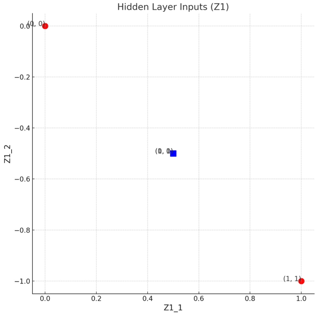
Input	Hidden Layer Inputs (\(\mathbf{Z}^{(1)}\))	Hidden Layer Outputs (\(\mathbf{A}^{(1)}\))	Output Layer Input (\(\mathbf{Z}^{(2)}\))	Output (\(\mathbf{y}\))
(1, 0)	\((0.5, -0.5)\)	\((0.462, -0.462)\)	\(0\)	\(0.5\)
(0, 1)	\((0.5, -0.5)\)	\((0.462, -0.462)\)	\(0\)	\(0.5\)
(0, 0)	\((0, 0)\)	\((0, 0)\)	\(0\)	\(0.5\)
(1, 1)	\((1, -1)\)	\((0.762, -0.762)\)	\(0\)	\(0.5\)

Visualization of Non-Linearity

The following images show the transformation from the hidden layer inputs (\(\mathbf{Z}^{(1)}\)) to the hidden layer outputs (\(\mathbf{A}^{(1)}\)) after applying the tanh activation function.

Hidden Layer Inputs (Z1)

Figure 1: Hidden Layer Inputs – Linear Transformations

Hidden Layer Outputs (A1 – Tanh Activation)

Figure 2: Hidden Layer Outputs – Non-Linear Transformations

Conclusion

The comparison between the linear hidden layer inputs and the non-linear hidden layer outputs clearly illustrates how the non-linear activation function (tanh) transforms the input space into a non-linear output space. This transformation enables the neural network to form a non-linear decision boundary, which is crucial for solving problems like XOR where a simple linear decision boundary is insufficient.