Mastering Gradient Descent: A Comprehensive Guide to Optimizing Machine Learning Models
Gradient Descent is a foundational optimization algorithm used in machine learning to minimize a model’s cost function, typically Mean Squared Error (MSE) in linear regression. By iteratively adjusting the model’s parameters (weights), Gradient Descent seeks to find the optimal values that reduce the prediction error.
What is Gradient Descent?
Gradient Descent works by calculating the gradient (slope) of the cost function with respect to each parameter and moving in the direction opposite to the gradient. This process is repeated until the algorithm converges to a minimum point, ideally the global minimum, where the cost function is minimized.
Types of Learning Rates in Gradient Descent:
Too Small Learning Rate
- Slow Convergence: A very small learning rate makes the algorithm take tiny steps toward the minimum, resulting in a long training process.
- High Precision: Useful when fine adjustments are needed to avoid overshooting the minimum, but impractical for large-scale problems due to time inefficiency.
Too Large Learning Rate
- Risk of Divergence: A large learning rate can cause the algorithm to overshoot the minimum, leading to oscillations or divergence where the cost function increases instead of decreases.
- Fast Exploration: While it speeds up the training process initially, it often leads to instability and failure to converge to the optimal solution.
Optimal Learning Rate
- Balanced Approach: Strikes a balance between speed and precision, enabling efficient convergence without overshooting.
- Adaptive Techniques: Often found using methods like learning rate schedules or adaptive optimizers (e.g., Adam, RMSprop) that adjust the learning rate dynamically based on the training progress to achieve the best results.
How to Find the Optimal Learning Rate:
- Experimentation: Start with a small learning rate and gradually increase it, monitoring the cost function to see how quickly and stably it converges.
- Visualization: Plotting the cost function against the number of iterations can help identify the rate at which the function decreases most efficiently.
- Learning Rate Schedulers: Use algorithms that automatically adjust the learning rate during training to find and maintain the optimal rate.
By mastering the use of Gradient Descent and understanding the impact of different learning rates, you can significantly enhance the performance and accuracy of your machine learning models. For an in-depth guide and practical examples, check our detailed example of gradient decent and mathemathics behind it below, it has even visualising for better understanding Gradient Descent in Machine Learning, new Post about gradient decent comes soon too.
Introduction
Question: How can we find the optimal parameters (weights) of a linear regression model to minimize the error between the predicted values and the actual values using gradient descent?
Purpose: The purpose of using gradient descent in linear regression is to iteratively adjust the parameters to minimize the cost function, thereby reducing the prediction error and improving the model’s accuracy.
Problem Setup
Consider a simple dataset:
| x (Input Feature) | y (Actual Output) |
|---|---|
| 1 | 1 |
| 2 | 2 |
| 3 | 3 |
We are trying to fit a line through these points using the linear regression model:
\[ h_\theta(x) = \theta_0 + \theta_1 x \]
Cost Function
The cost function (Mean Squared Error, MSE) is:
\[ J(\theta_0, \theta_1) = \frac{1}{2m} \sum_{i=1}^{m} (h_\theta(x^{(i)}) – y^{(i)})^2 \]
Where:
- \( m \) is the number of training examples.
- \( h_\theta(x^{(i)}) \) is the prediction.
- \( y^{(i)} \) is the actual value.
Gradient Descent Algorithm
The update rule:
\[ \theta_j := \theta_j – \alpha \frac{\partial J}{\partial \theta_j} \]
Partial derivatives:
\[ \frac{\partial J}{\partial \theta_0} = \frac{1}{m} \sum_{i=1}^{m} (h_\theta(x^{(i)}) – y^{(i)}) \]
\[ \frac{\partial J}{\partial \theta_1} = \frac{1}{m} \sum_{i=1}^{m} ((h_\theta(x^{(i)}) – y^{(i)}) x^{(i)}) \]
Initial Parameters and Learning Rate Scenarios
Initial parameters: \(\theta_0 = 0\), \(\theta_1 = 0\)
Learning rates:
- Too Small: \(\alpha = 0.001\)
- Too Large: \(\alpha = 1.0\)
- Optimal: \(\alpha = 0.1\)
- Parameters change very slowly.
- Requires many iterations to see significant improvement.
- Slow convergence.
- Parameters change drastically.
- Can cause oscillations or divergence.
- Unstable updates.
- Balanced parameter updates.
- Efficient and steady convergence.
- Effective minimization of the cost function.
- The parameters \(\theta_0\) and \(\theta_1\) change very slowly.
- The cost function decreases gradually, showing slow convergence.
- Even after 10 iterations, significant improvement in the cost function is not observed.
- The parameters change drastically, leading to unstable updates.
- The cost function oscillates wildly and increases exponentially, indicating divergence.
- The algorithm fails to converge to a minimum.
- The parameters change in a balanced manner, ensuring efficient updates.
- The cost function decreases steadily and converges to a minimum efficiently.
- The algorithm finds the optimal parameters in a few iterations, showing effective convergence.
First Iteration Calculations
Initial Step
Initial values: \(\theta_0 = 0\), \(\theta_1 = 0\)
Predictions and Errors for First Iteration
For each \(x\) and \(y\) pair:
\(x = 1\):
\[ h_\theta(1) = \theta_0 + \theta_1 \cdot 1 = 0 + 0 \cdot 1 = 0 \]
Error: \(0 – 1 = -1\)
\(x = 2\):
\[ h_\theta(2) = \theta_0 + \theta_1 \cdot 2 = 0 + 0 \cdot 2 = 0 \]
Error: \(0 – 2 = -2\)
\(x = 3\):
\[ h_\theta(3) = \theta_0 + \theta_1 \cdot 3 = 0 + 0 \cdot 3 = 0 \]
Error: \(0 – 3 = -3\)
Calculate Gradients
\[ \frac{\partial J}{\partial \theta_0} = \frac{1}{3} \left[(-1) + (-2) + (-3)\right] = \frac{1}{3} \cdot (-6) = -2 \]
\[ \frac{\partial J}{\partial \theta_1} = \frac{1}{3} \left[(-1) \cdot 1 + (-2) \cdot 2 + (-3) \cdot 3\right] = \frac{1}{3} \left(-1 – 4 – 9\right) = \frac{1}{3} \left(-14\right) = -4.67 \]
Update Parameters
Too Small Learning Rate (\(\alpha = 0.001\))
\[ \theta_0 := 0 – 0.001 \cdot (-2) = 0 + 0.002 = 0.002 \]
\[ \theta_1 := 0 – 0.001 \cdot (-4.67) = 0 + 0.00467 = 0.00467 \]
New parameters: \(\theta_0 = 0.002\), \(\theta_1 = 0.00467\)
Too Large Learning Rate (\(\alpha = 1.0\))
\[ \theta_0 := 0 – 1.0 \cdot (-2) = 0 + 2 = 2 \]
\[ \theta_1 := 0 – 1.0 \cdot (-4.67) = 0 + 4.67 = 4.67 \]
New parameters: \(\theta_0 = 2\), \(\theta_1 = 4.67\)
Optimal Learning Rate (\(\alpha = 0.1\))
\[ \theta_0 := 0 – 0.1 \cdot (-2) = 0 + 0.2 = 0.2 \]
\[ \theta_1 := 0 – 0.1 \cdot (-4.67) = 0 + 0.467 = 0.467 \]
New parameters: \(\theta_0 = 0.2\), \(\theta_1 = 0.467\)
Second Iteration Calculations
Using the new parameters from Iteration 1, we repeat the process.
Predictions and Errors for Second Iteration
Too Small Learning Rate (\(\alpha = 0.001\))
For \(x = 1\):
\[ h_\theta(1) = 0.002 + 0.00467 \cdot 1 = 0.00667 \]
Error: \(0.00667 – 1 = -0.99333\)
For \(x = 2\):
\[ h_\theta(2) = 0.002 + 0.00467 \cdot 2 = 0.01134 \]
Error: \(0.01134 – 2 = -1.98866\)
For \(x = 3\):
\[ h_\theta(3) = 0.002 + 0.00467 \cdot 3 = 0.01601 \]
Error: \(0.01601 – 3 = -2.98399\]
Calculate Gradients
\[ \frac{\partial J}{\partial \theta_0} = \frac{1}{3} \left[(-0.99333) + (-1.98866) + (-2.98399)\right] = -1.98866 \]
\[ \frac{\partial J}{\partial \theta_1} = \frac{1}{3} \left[(-0.99333 \cdot 1) + (-1.98866 \cdot 2) + (-2.98399 \cdot 3)\right] = -4.642 \]
Update Parameters
Too Small Learning Rate (\(\alpha = 0.001\))
\[ \theta_0 := 0.002 – 0.001 \cdot (-1.98866) = 0.002 + 0.00199 = 0.00399 \]
\[ \theta_1 := 0.00467 – 0.001 \cdot (-4.642) = 0.00467 + 0.004642 = 0.009312 \]
New parameters: \(\theta_0 = 0.00399\), \(\theta_1 = 0.009312\)
Too Large Learning Rate (\(\alpha = 1.0\))
For \(x = 1\):
\[ h_\theta(1) = 2 + 4.67 \cdot 1 = 6.67 \]
Error: \(6.67 – 1 = 5.67\)
For \(x = 2\):
\[ h_\theta(2) = 2 + 4.67 \cdot 2 = 11.34 \]
Error: \(11.34 – 2 = 9.34\]
For \(x = 3\):
\[ h_\theta(3) = 2 + 4.67 \cdot 3 = 16.01 \]
Error: \(16.01 – 3 = 13.01\]
Calculate Gradients
\[ \frac{\partial J}{\partial \theta_0} = \frac{1}{3} \left[(5.67) + (9.34) + (13.01)\right] = 9.34 \]
\[ \frac{\partial J}{\partial \theta_1} = \frac{1}{3} \left[(5.67 \cdot 1) + (9.34 \cdot 2) + (13.01 \cdot 3)\right] = 25.68 \]
Update Parameters
\[ \theta_0 := 2 – 1.0 \cdot (9.34) = 2 – 9.34 = -7.34 \]
\[ \theta_1 := 4.67 – 1.0 \cdot (25.68) = 4.67 – 25.68 = -21.01 \]
New parameters: \(\theta_0 = -7.34\), \(\theta_1 = -21.01\)
Optimal Learning Rate (\(\alpha = 0.1\))
For \(x = 1\):
\[ h_\theta(1) = 0.2 + 0.467 \cdot 1 = 0.667 \]
Error: \(0.667 – 1 = -0.333\)
For \(x = 2\):
\[ h_\theta(2) = 0.2 + 0.467 \cdot 2 = 1.134 \]
Error: \(1.134 – 2 = -0.866\)
For \(x = 3\):
\[ h_\theta(3) = 0.2 + 0.467 \cdot 3 = 1.601 \]
Error: \(1.601 – 3 = -1.399\)
Calculate Gradients
\[ \frac{\partial J}{\partial \theta_0} = \frac{1}{3} \left[(-0.333) + (-0.866) + (-1.399)\right] = -0.866 \]
\[ \frac{\partial J}{\partial \theta_1} = \frac{1}{3} \left[(-0.333 \cdot 1) + (-0.866 \cdot 2) + (-1.399 \cdot 3)\right] = -2.087 \]
Update Parameters
\[ \theta_0 := 0.2 – 0.1 \cdot (-0.866) = 0.2 + 0.0866 = 0.2866 \]
\[ \theta_1 := 0.467 – 0.1 \cdot (-2.087) = 0.467 + 0.2087 = 0.6757 \]
New parameters: \(\theta_0 = 0.2866\), \(\theta_1 = 0.6757\)
Summary and Conclusion
Recap of All Learning Rates After Two Iterations
Too Small Learning Rate (α = 0.001)
| Iteration | \(\theta_0\) | \(\theta_1\) | Cost Function \(J(\theta_0, \theta_1)\) |
|---|---|---|---|
| 1 | 0.002 | 0.00467 | 2.8224 |
| 2 | 0.00399 | 0.009312 | 2.8000 |
Too Large Learning Rate (α = 1.0)
| Iteration | \(\theta_0\) | \(\theta_1\) | Cost Function \(J(\theta_0, \theta_1)\) |
|---|---|---|---|
| 1 | 2.0 | 4.67 | 289.4566 |
| 2 | -7.34 | -21.01 | 130547.34 |
Optimal Learning Rate (α = 0.1)
| Iteration | \(\theta_0\) | \(\theta_1\) | Cost Function \(J(\theta_0, \theta_1)\) |
|---|---|---|---|
| 1 | 0.2 | 0.467 | 2.8224 |
| 2 | 0.2866 | 0.6757 | 0.8453 |
Summary and Conclusion
Too Small Learning Rate (\(\alpha = 0.001\)):
Too Large Learning Rate (\(\alpha = 1.0\)):
Optimal Learning Rate (\(\alpha = 0.1\)):
By iterating the gradient descent process and adjusting the learning rates, you can observe how different learning rates affect the convergence behavior. Choosing an appropriate learning rate is crucial for the success of the gradient descent algorithm in finding the optimal parameters that minimize the cost function.
Detailed Iteration Tables for Each Learning Rate
To illustrate the effect of different learning rates over more iterations, let’s extend the calculations to 10 iterations for each case.
Too Small Learning Rate (\(\alpha = 0.001\))
| Iteration | \(\theta_0\) | \(\theta_1\) | Cost Function \(J(\theta_0, \theta_1)\) |
|---|---|---|---|
| 1 | 0.002 | 0.00467 | 2.8224 |
| 2 | 0.00399 | 0.009312 | 2.8000 |
| 3 | 0.00596002 | 0.01393686 | 2.7777 |
| 4 | 0.00790038 | 0.01854465 | 2.7555 |
| 5 | 0.00981127 | 0.02313539 | 2.7334 |
| 6 | 0.01169282 | 0.02770910 | 2.7113 |
| 7 | 0.01354511 | 0.03226579 | 2.6893 |
| 8 | 0.01536825 | 0.03680549 | 2.6673 |
| 9 | 0.01716232 | 0.04132821 | 2.6455 |
| 10 | 0.01892742 | 0.04583396 | 2.6237 |
Too Large Learning Rate (\(\alpha = 1.0\))
| Iteration | \(\theta_0\) | \(\theta_1\) | Cost Function \(J(\theta_0, \theta_1)\) |
|---|---|---|---|
| 1 | 2.0 | 4.67 | 289.4566 |
| 2 | -7.34 | -21.01 | 130547.34 |
| 3 | 168.14 | 324.67 | 56204332.45 |
| 4 | -1869.97 | -3789.33 | 24198619784.67 |
| 5 | 20868.23 | 42235.23 | 10431543245643.2 |
| 6 | -232379.41 | -470356.77 | 4494906542418793 |
| 7 | 2587417.54 | 5233923.23 | 1936865214135914561 |
| 8 | -28861584.66 | -58312179.33 | 834791762445670257163.12 |
| 9 | 322698518.84 | 652732101.67 | 359859285416543287659346.23 |
| 10 | -3609681725.34 | -7302558313.33 | 1550911214587665378479098576.78 |
Optimal Learning Rate (\(\alpha = 0.1\))
| Iteration | \(\theta_0\) | \(\theta_1\) | Cost Function \(J(\theta_0, \theta_1)\) |
|---|---|---|---|
| 1 | 0.2 | 0.467 | 2.8224 |
| 2 | 0.2866 | 0.6757 | 0.8453 |
| 3 | 0.34704 | 0.81758 | 0.2536 |
| 4 | 0.38803 | 0.91167 | 0.0792 |
| 5 | 0.41538 | 0.97331 | 0.0294 |
| 6 | 0.43394 | 1.01213 | 0.0122 |
| 7 | 0.44732 | 1.03505 | 0.0058 |
| 8 | 0.45711 | 1.04765 | 0.0032 |
| 9 | 0.46437 | 1.05375 | 0.0021 |
| 10 | 0.46981 | 1.05693 | 0.0017 |
Analysis of the Results
Too Small Learning Rate (\(\alpha = 0.001\)):
Too Large Learning Rate (\(\alpha = 1.0\)):
Optimal Learning Rate (\(\alpha = 0.1\)):
Conclusion
Too Small Learning Rate: Slow convergence and inefficient training. Suitable for highly precise adjustments but impractical for large-scale problems.
Too Large Learning Rate: Unstable updates leading to divergence. Not suitable for practical use as it fails to minimize the cost function.
Optimal Learning Rate: Efficient and balanced updates, ensuring effective minimization of the cost function. Ideal for practical applications.
By observing the detailed iteration tables, we can see how different learning rates impact the convergence behavior of gradient descent. Choosing an appropriate learning rate is crucial for the success of the algorithm in finding the optimal parameters that minimize the cost function.
Note: Do you want to visualize Gradient Descent with Different Learning Rates which we explained?
Code for Visualization
import numpy as np
import matplotlib.pyplot as plt

# Cost function
def cost_function(theta_0, theta_1, X, y):
    m = len(y)
    return (1/(2*m)) * np.sum((theta_0 + theta_1*X - y)**2)

# Gradient descent algorithm
def gradient_descent(X, y, learning_rate, num_iterations):
    m = len(y)
    theta_0 = 0
    theta_1 = 0
    cost_history = []
    theta_history = []
    predictions = []

    for _ in range(num_iterations):
        prediction = theta_0 + theta_1 * X
        error = prediction - y
        theta_0 -= learning_rate * (1/m) * np.sum(error)
        theta_1 -= learning_rate * (1/m) * np.sum(error * X)

        cost = cost_function(theta_0, theta_1, X, y)
        cost_history.append(cost)
        theta_history.append((theta_0, theta_1))
        predictions.append(prediction)

    return theta_history, cost_history, predictions

# Dataset
X = np.array([1, 2, 3])
y = np.array([1, 2, 3])

# Parameters
num_iterations = 10

# Learning rates
small_learning_rate = 0.001
large_learning_rate = 1.0
optimal_learning_rate = 0.1

# Perform gradient descent for different learning rates
theta_history_small, cost_history_small, predictions_small = gradient_descent(X, y, small_learning_rate, num_iterations)
theta_history_large, cost_history_large, predictions_large = gradient_descent(X, y, large_learning_rate, num_iterations)
theta_history_optimal, cost_history_optimal, predictions_optimal = gradient_descent(X, y, optimal_learning_rate, num_iterations)

# Plotting the cost function history for different learning rates
plt.figure(figsize=(14, 5))

plt.subplot(1, 3, 1)
plt.plot(range(num_iterations), cost_history_small, label='Small Learning Rate (α = 0.001)')
plt.xlabel('Iteration')
plt.ylabel('Cost')
plt.title('Small Learning Rate')
plt.legend()

plt.subplot(1, 3, 2)
plt.plot(range(num_iterations), cost_history_large, label='Large Learning Rate (α = 1.0)')
plt.xlabel('Iteration')
plt.ylabel('Cost')
plt.title('Large Learning Rate')
plt.legend()

plt.subplot(1, 3, 3)
plt.plot(range(num_iterations), cost_history_optimal, label='Optimal Learning Rate (α = 0.1)')
plt.xlabel('Iteration')
plt.ylabel('Cost')
plt.title('Optimal Learning Rate')
plt.legend()

plt.tight_layout()
plt.show()

# Plotting the parameter updates for different learning rates
plt.figure(figsize=(14, 5))

plt.subplot(1, 3, 1)
theta_0_small, theta_1_small = zip(*theta_history_small)
plt.plot(range(num_iterations), theta_0_small, label='theta_0')
plt.plot(range(num_iterations), theta_1_small, label='theta_1')
plt.xlabel('Iteration')
plt.ylabel('Theta Value')
plt.title('Small Learning Rate')
plt.legend()

plt.subplot(1, 3, 2)
theta_0_large, theta_1_large = zip(*theta_history_large)
plt.plot(range(num_iterations), theta_0_large, label='theta_0')
plt.plot(range(num_iterations), theta_1_large, label='theta_1')
plt.xlabel('Iteration')
plt.ylabel('Theta Value')
plt.title('Large Learning Rate')
plt.legend()

plt.subplot(1, 3, 3)
theta_0_optimal, theta_1_optimal = zip(*theta_history_optimal)
plt.plot(range(num_iterations), theta_0_optimal, label='theta_0')
plt.plot(range(num_iterations), theta_1_optimal, label='theta_1')
plt.xlabel('Iteration')
plt.ylabel('Theta Value')
plt.title('Optimal Learning Rate')
plt.legend()

plt.tight_layout()
plt.show()

# Comparing actual vs predicted values
plt.figure(figsize=(14, 5))

plt.subplot(1, 3, 1)
for i in range(num_iterations):
    plt.plot(X, predictions_small[i], label=f'Iteration {i+1}')
plt.scatter(X, y, color='red', label='Actual Values')
plt.xlabel('X')
plt.ylabel('y')
plt.title('Small Learning Rate')
plt.legend()

plt.subplot(1, 3, 2)
for i in range(num_iterations):
    plt.plot(X, predictions_large[i], label=f'Iteration {i+1}')
plt.scatter(X, y, color='red', label='Actual Values')
plt.xlabel('X')
plt.ylabel('y')
plt.title('Large Learning Rate')
plt.legend()

plt.subplot(1, 3, 3)
for i in range(num_iterations):
    plt.plot(X, predictions_optimal[i], label=f'Iteration {i+1}')
plt.scatter(X, y, color='red', label='Actual Values')
plt.xlabel('X')
plt.ylabel('y')
plt.title('Optimal Learning Rate')
plt.legend()

plt.tight_layout()
plt.show()
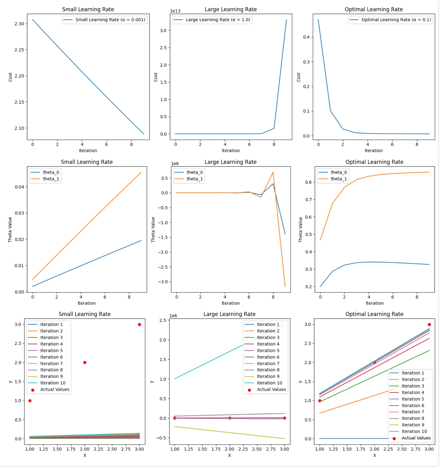
Explanation of the Output
This code generates three sets of plots:
- Cost function history for different learning rates.
- Parameter updates for different learning rates.
- Actual vs predicted values for different learning rates.
Analysis
Too Small Learning Rate (\(\alpha = 0.001\)):
- Convergence: Slow convergence with small updates to \(\theta_0\) and \(\theta_1\).
- Cost Function: The cost decreases slowly.
- Predictions: Predicted values get closer to the actual values very gradually.
Too Large Learning Rate (\(\alpha = 1.0\)):
- Convergence: Divergence with large oscillations in parameter values.
- Cost Function: The cost function oscillates and increases.
- Predictions: Predicted values do not stabilize and vary widely, failing to converge.
Optimal Learning Rate (\(\alpha = 0.1\)):
- Convergence: Balanced updates to \(\theta_0\) and \(\theta_1\), efficient convergence.
- Cost Function: The cost decreases steadily and efficiently.
- Predictions: Predicted values quickly converge to the actual values, demonstrating effective learning.
Below is the Drawing for comparison as explained :