Fine-Tuning in Deep Learning with a practical example – day 6

November 5, 2024
Posted by ingoampt

Understanding Fine-Tuning in Deep Learning

Understanding Fine-Tuning in Deep Learning: A Comprehensive Overview

Fine-tuning in deep learning has become a powerful technique, allowing developers to adapt pre-trained models to specific tasks without training from scratch. This approach is especially valuable in areas like natural language processing, computer vision, and voice cloning. In this article, we’ll explore what fine-tuning is, why it’s used, how it works from mathematical and neural perspectives, and provide a practical implementation as well.

What is Fine-Tuning in Deep Learning?

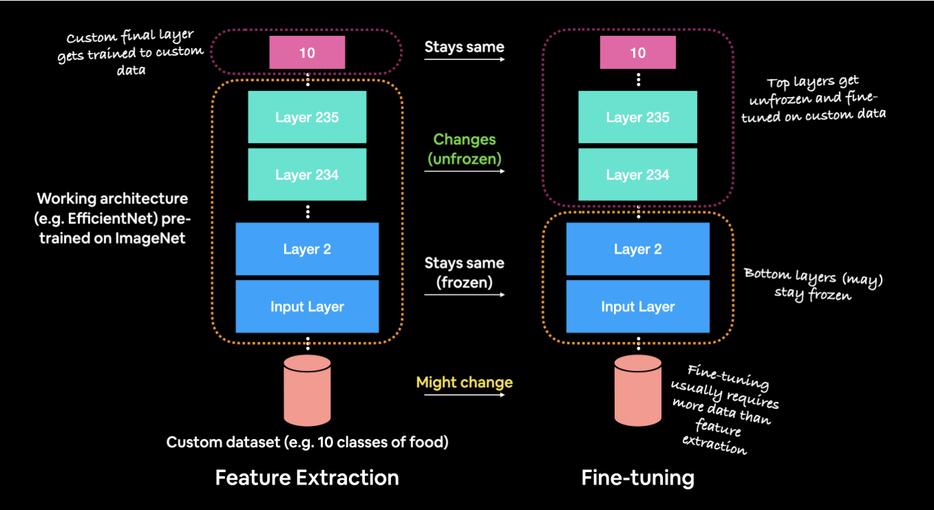
Fine-tuning is the process of taking a pre-trained model (a model trained on a large, general dataset) and adapting it to a specific, smaller dataset. This allows the model to retain its general knowledge and refine it to fit a new, task-specific context. For example, a voice synthesis model can be fine-tuned to replicate a specific person’s voice.

Why Fine-Tuning?

Fine-tuning is beneficial for several reasons:

Benefit	Description
Efficiency	Saves time and computational power by leveraging pre-trained models.
Knowledge Transfer	Retains general patterns learned from large datasets and applies them to a new context.
Transfer Learning	Uses insights from one task (e.g., general speech synthesis) to perform related tasks (e.g., mimicking a new voice).

How Does Fine-Tuning Work?

The fine-tuning process can be broken down into several steps:

1. Selecting a Pre-Trained Model

Choose a model pre-trained on a large, general dataset relevant to the target domain. Examples include Tacotron 2 or WaveGlow for speech synthesis tasks.

2. Modify the Model Architecture

Adjust the final layers to fit the new task. For instance, add a new layer to adapt a general model to a specific speaker in voice cloning.

3. Freeze Layers

Freezing lower layers prevents overwriting general features. This keeps early layers that capture basic features (like phonemes) intact, focusing fine-tuning on task-specific features.

4. Training on Task-Specific Data

Only a portion of the model’s layers are trainable, which means the model only learns new patterns relevant to the new dataset, preserving pre-trained knowledge.

5. Evaluation and Optimization

After training, evaluate the model’s performance and adjust hyperparameters as needed.

Benefits and Challenges of Fine-Tuning

Benefits

Benefit	Explanation
Efficient Training	Faster and less resource-intensive than training from scratch.
Specialization	Can adapt a general-purpose model to perform highly specialized tasks.
Robustness	Combines the pre-trained model’s generalization with task-specific learning for better performance.

Challenges

Challenge	Explanation
Data Scarcity	Limited data in certain domains can make fine-tuning difficult.
Overfitting	Risk of overfitting to a small, specific dataset.
Quality Retention	Fine-tuning must ensure that the model’s general capabilities are not degraded in the process.

Mathematical Foundations of Fine-Tuning: Why It Works

Fine-tuning is effective due to mathematical principles around parameter optimization and regularization. Below are key mathematical concepts that underpin why fine-tuning works:

1. Parameter Space and Loss Function

Fine-tuning works by optimizing a loss function $L(\theta)$ that measures the difference between the model’s predictions and the target outputs. The parameters $\theta_{\text{pre-trained}}$ in a pre-trained model are already close to a minimum for the general task (e.g., speech synthesis), making fine-tuning computationally efficient.

Objective in Fine-Tuning:

$\theta^* = \arg \min_{\theta} L_{\text{target}}(\theta)$
where $\theta = \theta_{\text{pre-trained}} + \Delta \theta$ .

This formula shows that fine-tuning involves adjusting $\Delta \theta$ (the changes to the original pre-trained parameters) to minimize the task-specific loss $L_{\text{target}}$ .

2. Optimization Landscape

In deep learning, training from scratch requires navigating a large optimization landscape to find an optimal minimum. Fine-tuning, however, begins with parameters already near a good local minimum because they were optimized for a similar task, such as general speech synthesis.

Training Approach	Optimization Requirement
From Scratch	Find an optimal point in a large parameter space.
Fine-Tuning	Start near a minimum and make small adjustments for the new task.

3. Regularization through Constrained Optimization

Fine-tuning can be viewed as a form of regularization that constrains the model from deviating too far from the pre-trained parameters. Mathematically, this is often achieved by adding a regularization term to the loss function:

$L_{\text{fine-tune}}(\theta) = L_{\text{target}}(\theta) + \lambda \| \theta - \theta_{\text{pre-trained}} \|^2$

This regularization ensures that fine-tuning doesn’t drastically alter the model, which helps prevent overfitting to the smaller task-specific dataset.

4. Transfer Learning Theory and Generalization

Fine-tuning is effective because it leverages transfer learning principles. The pre-trained model contains useful features learned from a large, diverse dataset. By adjusting the higher layers during fine-tuning, these generalized features are adapted to a new, more specific task without needing to retrain the entire network.

Transfer Learning Assumption: If the source and target tasks share underlying structures, then:

$L_{\text{source}}(\theta) \approx L_{\text{target}}(\theta)$

—

Neural Network Perspective on Fine-Tuning

From a neural network perspective, fine-tuning works due to the hierarchical feature structure within the layers:

1. Feature Hierarchies

Lower layers capture general features, like edges in images or phonemes in speech, which are transferable across tasks. These are often “frozen” during fine-tuning to retain their general knowledge. Higher layers are “trainable” during fine-tuning to adapt to the target task.

2. Representational Knowledge Transfer

The pre-trained model contains rich representations from its initial training, which can be adapted to the specific characteristics of the new task. Fine-tuning then modifies only the necessary parameters, allowing the model to specialize in the target task without sacrificing the general knowledge it has acquired.

3. Fine-Tuning in Transformers

In Transformers, fine-tuning involves adjusting the self-attention layers to focus on task-specific relationships and adding task-specific heads, like classification heads for sentiment analysis.

Fine-Tuning a Voice Cloning Model Using PyTorch

Fine-Tuning a Voice Cloning Model Using PyTorch: Step-by-Step Guide

Overview of Voice Cloning and Required Data

Voice cloning involves generating synthetic speech that mimics the characteristics of a target speaker’s voice. For this, you need:

Audio recordings of the target speaker: The data should cover a wide range of sounds and tones, ideally with high audio quality.
Transcriptions: Accurate transcriptions are essential to match the spoken content with the audio for model training.

Data Sources for Voice Cloning

There are several ways to source data for voice cloning:

Public Datasets: Datasets like LibriSpeech and VCTK provide extensive recordings of various speakers.
Custom Data Collection: If the target speaker is someone specific, such as a client or public figure, you may need to collect custom recordings in a quiet environment with high-quality recording devices.

Purpose of Data: The data provides the model with examples of how the target speaker pronounces words, uses tone, and varies pitch. This information is crucial for the model to understand and replicate the nuances of the speaker’s voice.

—

Step 1: Environment Setup

Objective: Set up the environment by installing PyTorch and essential libraries like NumPy and Librosa for audio processing.

# Install PyTorch
pip install torch torchvision torchaudio

# Install additional dependencies
pip install numpy librosa

Explanation: We use PyTorch as our deep learning framework, while NumPy handles numerical operations, and Librosa is a popular library for audio processing.

—

Step 2: Data Collection and Preprocessing

Objective: Collect and preprocess audio recordings from the target speaker.

Data Preprocessing Steps

Normalization: Adjust the volume of all audio files to a consistent level.
Trimming Silence: Remove silent parts from the beginning and end of each audio file.
Resampling: Ensure all audio files have the same sampling rate (usually 22,050 Hz for voice cloning).

import librosa
import numpy as np

def preprocess_audio(file_path):
    # Load audio file
    y, sr = librosa.load(file_path, sr=22050)  # Resample to 22,050 Hz
    # Normalize volume
    y = librosa.util.normalize(y)
    # Trim silence
    y, _ = librosa.effects.trim(y)
    return y, sr

Explanation: Preprocessing the audio ensures consistency, allowing the model to learn more effectively without being influenced by volume differences or silent gaps.

—

Step 3: Feature Extraction

Objective: Convert audio data into features that the model can learn from. Typically, Mel-spectrograms are used for voice cloning.

Why Mel-Spectrograms?

A Mel-spectrogram represents audio in terms of time and frequency, showing how sound energy varies across different frequencies over time. This format is more interpretable for deep learning models than raw audio data.

def extract_mel_spectrogram(y, sr):
    # Compute mel-spectrogram
    mel_spec = librosa.feature.melspectrogram(y, sr=sr, n_mels=80)
    # Convert to decibel scale
    mel_spec_db = librosa.power_to_db(mel_spec, ref=np.max)
    return mel_spec_db

Explanation: The Mel-spectrogram condenses audio information into a visual format that captures pitch, tone, and intensity, making it suitable for the model to learn the unique characteristics of the speaker’s voice.

—

Step 4: Model Selection

Objective: Load a pre-trained model suitable for voice cloning, such as Tacotron 2 (for generating Mel-spectrograms from text) and WaveGlow (for converting Mel-spectrograms to audio).

Why Use Tacotron 2 and WaveGlow?

Tacotron 2 synthesizes Mel-spectrograms based on text input, enabling the model to learn pronunciation and rhythm. WaveGlow acts as a vocoder, converting Mel-spectrograms to audio, giving the synthetic speech a natural, human-like quality.

import torch
from tacotron2 import Tacotron2
from waveglow import WaveGlow

# Load pre-trained models
tacotron2 = Tacotron2()
waveglow = WaveGlow()

# Load pre-trained weights
tacotron2.load_state_dict(torch.load('tacotron2_statedict.pt'))
waveglow.load_state_dict(torch.load('waveglow_statedict.pt'))

Explanation: Loading pre-trained models helps avoid training from scratch, saving computational resources and leveraging knowledge from large datasets.

—

Step 5: Fine-Tuning the Model

Objective: Fine-tune the model on your specific dataset by training only the higher layers. This step allows the model to adjust to the target speaker’s characteristics while retaining general knowledge about speech.

Steps for Fine-Tuning

Freeze Lower Layers: Lock the parameters of the lower layers so they don’t change during fine-tuning.
Set Up the Optimizer: Define an optimizer to update only the trainable layers.
Training Loop: Adjust the model parameters to minimize the error between generated and target Mel-spectrograms for each batch.

# Freeze lower layers
for param in tacotron2.encoder.parameters():
    param.requires_grad = False

# Define optimizer
optimizer = torch.optim.Adam(filter(lambda p: p.requires_grad, tacotron2.parameters()), lr=1e-4)

# Training loop
for epoch in range(num_epochs):
    for mel_spec, text in dataloader:
        optimizer.zero_grad()
        outputs = tacotron2(text, mel_spec)
        loss = loss_function(outputs, mel_spec)
        loss.backward()
        optimizer.step()

Explanation: By only updating specific layers, we ensure that the model adapts to the speaker’s voice characteristics while retaining general knowledge of speech sounds.

—

Step 6: Synthesize Speech

Objective: Test the fine-tuned model by synthesizing speech from text. This step generates audio outputs based on given text, allowing you to evaluate the model’s effectiveness.

def synthesize_speech(text):
    # Convert text to sequence
    sequence = text_to_sequence(text)
    # Generate mel-spectrogram
    mel_outputs, _, _ = tacotron2.inference(sequence)
    # Generate audio
    audio = waveglow.infer(mel_outputs)
    return audio

# Example usage
text = &quot;Hello, this is a voice cloning example.&quot;
audio = synthesize_speech(text)

Explanation: This function converts input text into an audio waveform using the fine-tuned model, making it possible to generate synthetic speech.

—

Step 7: Evaluate the Model

Objective: Assess the quality of the synthesized speech to ensure it matches the target voice.

Evaluation Techniques

Mean Opinion Score (MOS): A subjective rating from human listeners to evaluate audio quality.
Spectrogram Comparison: Compare Mel-spectrograms of generated and target audio to visually inspect quality and similarity.

import matplotlib.pyplot as plt

def plot_spectrogram(mel_spec):
    plt.figure(figsize=(10, 4))
    plt.imshow(mel_spec, aspect='auto', origin='lower')
    plt.colorbar()
    plt.title('Mel-Spectrogram')
    plt.show()

# Plot original and synthesized spectrograms
plot_spectrogram(original_mel_spec)
plot_spectrogram(synthesized_mel_spec)

Explanation: Visual and subjective evaluations ensure the synthesized voice matches the target speaker’s characteristics and meets quality expectations.

—

Conclusion

This detailed approach demonstrates how to fine-tune a pre-trained voice cloning model with PyTorch. By following each step carefully, you can customize a general model to replicate a specific speaker’s voice. Fine-tuning enables efficient model adaptation, leveraging pre-existing knowledge while learning new, task-specific nuances.

For further exploration, refer to the original Voice Cloning Techniques in PyTorch article.

Education