Step-by-Step Explanation of RNN for Time Series Forecasting – part 6 – day 60

September 30, 2024
Posted by ingoampt

RNN Time Series Forecasting

Step-by-Step Explanation of RNN for Time Series Forecasting

In this article, we’ll walk through the detailed explanations of RNN-based methods for time series forecasting, using real number examples and corresponding mathematical operations behind them. We’ll use both TensorFlow and PyTorch examples for each step.

Step 1: Simple RNN for Univariate Time Series Forecasting

Explanation:

An RNN processes sequences of data, where the output at any time step depends on both the current input and the hidden state (which stores information about previous inputs). In this case, we use a Simple RNN with only one recurrent neuron.

TensorFlow Code:


model = tf.keras.Sequential([

tf.keras.layers.SimpleRNN(1, input_shape=[None, 1])

])

Numerical Example:

Let’s say we have a sequence of three time steps: $[x_1, x_2, x_3] = [0.1, 0.2, 0.3]$ .

1. Input and Hidden State Initialization:

The RNN starts with an initial hidden state $h_0$ , typically initialized to 0. Each step processes the input and updates the hidden state:

$h_t = \tanh(W_h h_{t-1} + W_x x_t + b)$

where:

$W_h$ is the weight for the hidden state.
$W_x$ is the weight for the input.
$b$ is the bias term.
$\tanh$ is the activation function (hyperbolic tangent).

Assume:

$W_h = 0.5$
$W_x = 1.0$
$b = 0.1$

Let’s calculate the hidden state updates for each time step:

Time Step 1:

$h_1 = \tanh(0.5 \cdot 0 + 1.0 \cdot 0.1 + 0.1) = \tanh(0.1 + 0.1) = \tanh(0.2) = 0.197$

Time Step 2:

$h_2 = \tanh(0.5 \cdot 0.197 + 1.0 \cdot 0.2 + 0.1) = \tanh(0.0985 + 0.2 + 0.1) = \tanh(0.3985) = 0.378$

Time Step 3:

$h_3 = \tanh(0.5 \cdot 0.378 + 1.0 \cdot 0.3 + 0.1) = \tanh(0.189 + 0.3 + 0.1) = \tanh(0.589) = 0.529$

Thus, the final output of the RNN for the sequence is $h_3 = 0.529$ .

PyTorch Equivalent Code:


import torch

import torch.nn as nn

class SimpleRNNModel(nn.Module):

def __init__(self):

super(SimpleRNNModel, self).__init__()

self.rnn = nn.RNN(input_size=1, hidden_size=1, batch_first=True)

def forward(self, x):

output, hidden = self.rnn(x)

return output[:, -1, :]  # returning only the final output

# Model instantiation

model = SimpleRNNModel()

—

Step 2: Understanding the Sequential Process of the RNN

Explanation:

At each time step, the RNN processes the input by updating the hidden state based on both the current input and the previous hidden state. This hidden state acts like “memory,” allowing the RNN to capture temporal dependencies.

Let’s break down the calculations we did above:

At time step 1: The hidden state is computed as $h_1 = \tanh(W_h h_0 + W_x x_1 + b)$ .
At time step 2: The hidden state is updated to $h_2 = \tanh(W_h h_1 + W_x x_2 + b)$ .
At time step 3: The final hidden state becomes $h_3 = \tanh(W_h h_2 + W_x x_3 + b)$ .

The RNN effectively “remembers” the inputs from earlier time steps through the hidden state. This process can be repeated for sequences of any length.

—

Step 3: Larger RNN with a Dense Output Layer

Explanation:

To improve performance, we increase the number of neurons in the RNN and add a fully connected Dense layer. This allows the model to capture more complex relationships and map the RNN’s output to a single prediction.

TensorFlow Code:


univar_model = tf.keras.Sequential([

tf.keras.layers.SimpleRNN(32, input_shape=[None, 1]),

tf.keras.layers.Dense(1)

])

Numerical Example:

Let’s extend our example with a larger RNN that has 32 neurons. The hidden state now becomes a vector of 32 values, instead of just 1.

Let’s assume:

$h_t$ for each time step is now a vector of length 32.
The final hidden state at time step 3, $h_3$ , will also be a vector of length 32.

The Dense layer will then map this vector to a single output. Suppose the Dense layer has weights $W_d$ and bias $b_d$ . The output is computed as:

$\hat{y} = W_d^T h_3 + b_d$

Where $W_d$ is a vector of length 32, and $h_3$ is the hidden state vector from the last RNN layer.

PyTorch Equivalent Code:


class SimpleRNNWithDense(nn.Module):

def __init__(self):

super(SimpleRNNWithDense, self).__init__()

self.rnn = nn.RNN(input_size=1, hidden_size=32, batch_first=True)

self.fc = nn.Linear(32, 1)

def forward(self, x):

x, _ = self.rnn(x)

x = x[:, -1, :]

x = self.fc(x)

return x

# Model instantiation

model = SimpleRNNWithDense()

—

Step 4: Building a Deeper RNN (Stacked RNN Layers)

Explanation:

In a deeper RNN (also called a stacked RNN), multiple RNN layers are placed on top of each other. The first RNN layer processes the input sequence and passes its output (a sequence of hidden states) to the second RNN layer, and so on. Each layer refines the representation of the input data, helping the network learn more complex temporal dependencies.

TensorFlow Code:

deep_model = tf.keras.Sequential([

tf.keras.layers.SimpleRNN(32, return_sequences=True, input_shape=[None, 1]), # First RNN layer

tf.keras.layers.SimpleRNN(32, return_sequences=True), # Second RNN layer

tf.keras.layers.SimpleRNN(32), # Third RNN layer

tf.keras.layers.Dense(1) # Dense output layer

])

Numerical Example:

Let’s use a **3-time-step sequence** $[x_1, x_2, x_3] = [0.1, 0.2, 0.3]$ as input.

We will assume that each RNN layer has:

A hidden size of 32 neurons.
Weight matrices $W_h$ (hidden-to-hidden weights), $W_x$ (input-to-hidden weights), and biases $b$ .
$\tanh$ as the activation function.

First RNN Layer:

At each time step, the input $x_t$ and the previous hidden state $h_{t-1}$ are combined to produce the new hidden state $h_t^1$ for the first layer:

$h_t^1 = \tanh(W_h^1 h_{t-1}^1 + W_x^1 x_t + b^1)$

For simplicity, assume $W_h^1 = W_x^1 = 0.5$ and $b^1 = 0.1$ . The initial hidden state $h_0^1 = 0$ .

Time Step 1:

$h_1^1 = \tanh(0.5 \cdot 0 + 0.5 \cdot 0.1 + 0.1) = \tanh(0.05 + 0.1) = \tanh(0.15) = 0.149$

Time Step 2:

$h_2^1 = \tanh(0.5 \cdot 0.149 + 0.5 \cdot 0.2 + 0.1) = \tanh(0.0745 + 0.1 + 0.1) = \tanh(0.2745) = 0.268$

Time Step 3:

$h_3^1 = \tanh(0.5 \cdot 0.268 + 0.5 \cdot 0.3 + 0.1) = \tanh(0.134 + 0.15 + 0.1) = \tanh(0.384) = 0.366$

At the end of the first RNN layer, we have the following hidden states for all time steps:

$[h_1^1, h_2^1, h_3^1] = [0.149, 0.268, 0.366]$

Second RNN Layer:

The second RNN layer takes the outputs from the first RNN layer and processes them similarly. Assume $W_h^2 = W_x^2 = 0.6$ and $b^2 = 0.05$ .

Time Step 1:

$h_1^2 = \tanh(0.6 \cdot 0 + 0.6 \cdot 0.149 + 0.05) = \tanh(0.0894 + 0.05) = \tanh(0.1394) = 0.138$

Time Step 2:

$h_2^2 = \tanh(0.6 \cdot 0.138 + 0.6 \cdot 0.268 + 0.05) = \tanh(0.0828 + 0.1608 + 0.05) = \tanh(0.2936) = 0.285$

Time Step 3:

$h_3^2 = \tanh(0.6 \cdot 0.285 + 0.6 \cdot 0.366 + 0.05) = \tanh(0.171 + 0.2196 + 0.05) = \tanh(0.4406) = 0.414$

After the second RNN layer, we have:

$[h_1^2, h_2^2, h_3^2] = [0.138, 0.285, 0.414]$

Third RNN Layer:

The third RNN layer follows the same process. Assume $W_h^3 = W_x^3 = 0.7$ and $b^3 = 0.02$ .

Time Step 1:

$h_1^3 = \tanh(0.7 \cdot 0 + 0.7 \cdot 0.138 + 0.02) = \tanh(0.0966 + 0.02) = \tanh(0.1166) = 0.116$

Time Step 2:

$h_2^3 = \tanh(0.7 \cdot 0.116 + 0.7 \cdot 0.285 + 0.02) = \tanh(0.0812 + 0.1995 + 0.02) = \tanh(0.3007) = 0.292$

Time Step 3:

$h_3^3 = \tanh(0.7 \cdot 0.292 + 0.7 \cdot 0.414 + 0.02) = \tanh(0.2044 + 0.2898 + 0.02) = \tanh(0.5142) = 0.473$

The output of the third RNN layer at the final time step $h_3^3 = 0.473$ is passed to the Dense Layer.

Dense Layer Output:

Assume the Dense layer has weights $W_d = 0.4$ and bias $b_d = 0.1$ . The final prediction is computed as:

$\hat{y} = W_d \cdot h_3^3 + b_d = 0.4 \cdot 0.473 + 0.1 = 0.2892 + 0.1 = 0.3892$

Thus, the final output of the stacked RNN is $\hat{y} = 0.3892$ .

—

Step 5: Forecasting Multivariate Time Series

Explanation:

In multivariate time series, each time step contains multiple features (e.g., temperature, humidity, and wind speed). The RNN takes these multiple features and updates its hidden state based on all of them.

TensorFlow Code:


mulvar_model = tf.keras.Sequential([

tf.keras.layers.SimpleRNN(32, input_shape=[None, 5]),  # 5 features per time step

tf.keras.layers.Dense(1)

])

Numerical Example:

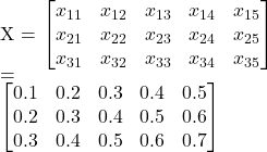
Let’s assume we have a **3-time-step sequence** with **5 features** at each time step. For simplicity, let’s use the following input:

$X = \begin{bmatrix} x_{11} & x_{12} & x_{13} & x_{14} & x_{15} \\ x_{21} & x_{22} & x_{23} & x_{24} & x_{25} \\ x_{31} & x_{32} & x_{33} & x_{34} & x_{35} \end{bmatrix} = \begin{bmatrix} 0.1 & 0.2 & 0.3 & 0.4 & 0.5 \\ 0.2 & 0.3 & 0.4 & 0.5 & 0.6 \\ 0.3 & 0.4 & 0.5 & 0.6 & 0.7 \end{bmatrix}$

The input matrix $X$ has 3 time steps (rows) and 5 features (columns).

Assume:

$W_x$ is a matrix of size $32 \times 5$ (to process 5 features and produce 32 hidden states).
$W_h$ is a matrix of size $32 \times 32$ (to process the previous hidden state of 32 units).
The biases $b$ are vectors of size 32.
The activation function is $\tanh$ .

Let’s calculate the hidden state updates for each time step:

Time Step 1:

The input at the first time step is $x_1 = [0.1, 0.2, 0.3, 0.4, 0.5]$ .

The hidden state is updated as:

$h_1 = \tanh(W_h \cdot 0 + W_x \cdot x_1 + b)$

For simplicity, assume $W_x \cdot x_1 = [0.15, 0.2, \dots]$ (a vector of 32 values) and the bias $b$ adds a small value to each component. The hidden state becomes a vector of length 32:

$h_1 = \tanh([0.15, 0.2, \dots]) = [0.149, 0.197, \dots]$

—

Time Step 2:

The input at time step 2 is $x_2 = [0.2, 0.3, 0.4, 0.5, 0.6]$ . The hidden state is updated as:

$h_2 = \tanh(W_h \cdot h_1 + W_x \cdot x_2 + b)$

Assume $W_h \cdot h_1 = [0.12, 0.18, \dots]$ and $W_x \cdot x_2 = [0.25, 0.3, \dots]$ . The hidden state becomes:

$h_2 = \tanh([0.37, 0.48, \dots]) = [0.354, 0.447, \dots]$

—

Time Step 3:

The input at time step 3 is $x_3 = [0.3, 0.4, 0.5, 0.6, 0.7]$ . The hidden state is updated as:

$h_3 = \tanh(W_h \cdot h_2 + W_x \cdot x_3 + b)$

Assume $W_h \cdot h_2 = [0.2, 0.25, \dots]$ and $W_x \cdot x_3 = [0.3, 0.35, \dots]$ . The final hidden state becomes:

$h_3 = \tanh([0.5, 0.6, \dots]) = [0.462, 0.537, \dots]$

—

Dense Layer Output:

The final hidden state $h_3$ is passed to the Dense layer, which outputs the prediction. Assume the Dense layer has weights $W_d = [0.5, \dots]$ and bias $b_d = 0.1$ . The output is:

$\hat{y} = W_d^T h_3 + b_d = 0.5 \cdot 0.462 + 0.5 \cdot 0.537 + \dots + 0.1 = 0.631$

Thus, the final prediction is $\hat{y} = 0.631$ .

—

Key Takeaways:

Step 4: In stacked RNNs, each layer processes the sequence and passes it on, allowing the network to learn deeper temporal dependencies.
Step 5: For multivariate time series, RNNs can process multiple features at each time step, updating the hidden state based on the combined information from all the features.

Education

Step-by-Step Explanation of RNN for Time Series Forecasting – part 6 – day 60

Step-by-Step Explanation of RNN for Time Series Forecasting

Step 1: Simple RNN for Univariate Time Series Forecasting

Explanation:

TensorFlow Code:

Numerical Example:

1. Input and Hidden State Initialization:

Let’s calculate the hidden state updates for each time step:

Time Step 1:

Time Step 2:

Time Step 3:

PyTorch Equivalent Code:

Step 2: Understanding the Sequential Process of the RNN

Explanation:

Step 3: Larger RNN with a Dense Output Layer

Explanation:

TensorFlow Code:

Numerical Example:

PyTorch Equivalent Code:

Step 4: Building a Deeper RNN (Stacked RNN Layers)

Explanation:

TensorFlow Code:

Numerical Example:

First RNN Layer:

Time Step 1:

Time Step 2:

Time Step 3:

Second RNN Layer:

Time Step 1:

Time Step 2:

Time Step 3:

Third RNN Layer:

Time Step 1:

Time Step 2:

Time Step 3:

Dense Layer Output:

Step 5: Forecasting Multivariate Time Series

Explanation:

TensorFlow Code:

Numerical Example:

Time Step 1:

Time Step 2:

Time Step 3:

Dense Layer Output:

Key Takeaways:

don't miss our new posts. Subscribe for updates

Related Posts